Synthesis
Two primary questions that motivated the initial study were:
Can geophysical data and 3D inversion delineate the various units shown in the geologic section?
The use of 3D inversion for interpreting with multiple physical properties was successful. Here, the Breakaway shale was a major conductor and the Moondarra siltstone a moderate one. However, the shale is unimportant for exploration in this region when compared to the Moondarra that hosts the Mt Novit Horizon. Once the induced polarization was introduced, it highlighted the Mt Hovit Horizon within the Moondarra and the mineralized zone in the Native Bee Siltstone. The shale is then exposed as just conductive and the main feature in the conductivity model is delineated as non-mineral bearing.
Can conductive and chargeable units, which would be potential targets, within the siltstones be identified?
The Mt Novit Horizon is characterized by a zone of moderately high conductivity and high chargeability. There is variation in amplitude and breakages, which could be a proxy to mineralization grade. The mineralization within the Native Bee Siltstone is also present in the model, albeit not as pronounced as the Mt Novit Horizon.
Additional questions were asked with the opportunity to re-invert the same data, but use improved algorithms and higher performance computers:
Are improved results obtained by using updated algorithms and higher performance computers?
The answer to this question is summarized using Fig. 459 and Fig. 460. These compare the recovered conductivity (Fig. 459) and chargeability (Fig. 460) models presented in [ROS01] with the updated model presented in this study. Both studies used identical datasets and inversion parameters, but finer horizontal cell-size discretization was 25 x 50 m compared to 40 x 100 m in the original study.s
Are there any lessons worth highlighting that arose within this case history that were not delineated in the initial case history paper?
One interesting feature in the recovered model is the conductor at the south-east edge of the model, which can be seen in Fig. 459. This feature is present in both the previous inversion and this case history. We further explore this conductor in the next section.
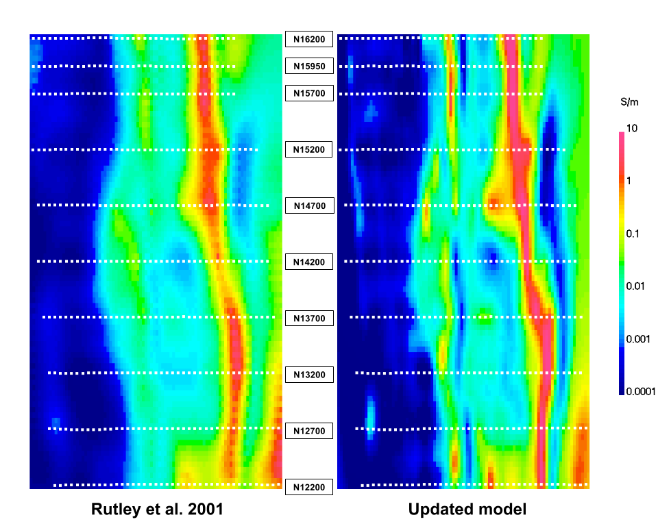
Fig. 459 Comparative sections through the recovered 3D conductivity model presented in [ROS01] (left) and this study (right).
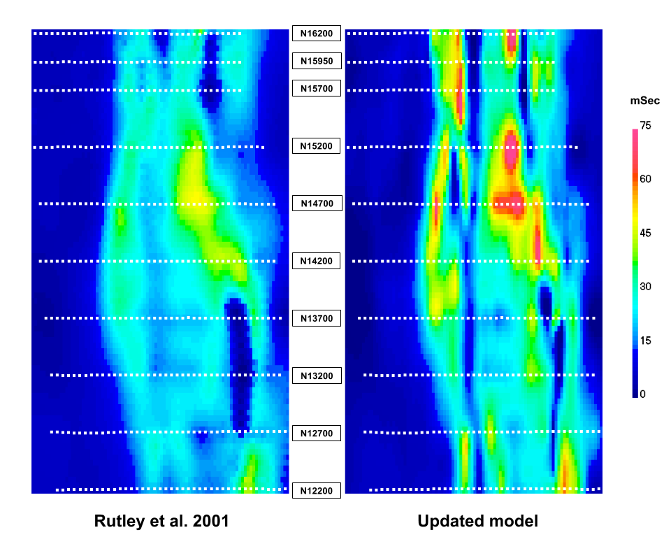
Fig. 460 Comparative sections through the recovered 3D chargeability model presented in [ROS01] (left) and this study (right).