This section provides an overview of the data quality control measures and
inversions completed on the Mt. Isa data sets. The DC data is first discussed.
The conductivity from those inversions are then used for IP inversions.
As presented in the previous section, the MIMDAS system
collects simultaneously a pole-dipole (P-DP) and a dipole-pole (DP-P) data
configuration. Accordingly, the P-DP and DP-P data were inverted separately in
2D. The uncertainties are assigned as 5% of the data amplitude with a minimum
floor value of 0.02 mV. The data were inverted and no noticeably bad data
points were obvious in the data misfit maps. This also means that data were
correctly normalized so they corresponded to a unit amplitude current in the
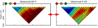
transmitter. The figure below shows the observed and
predicted data and recovered models for both configurations and for each of
the ten 2D lines. There are some regions where there are significant
differences in the conductivities obtained from the P-DP and DP-P
configurations. Some of this might be attributable to the fact that the two
surveys illuminate buried conductors quite differently due to current channeling.
Overall, however the inversion results have the same general distribution of
conductivity and there doesn not appear to be major issues with normalizations
or bad electrodes.
Table 14 : Independent 2D inversions of the P-DP and DP-P DCR data
Fig. 450 The P-DP and DP-P data sets are merged and then jointly inverted.
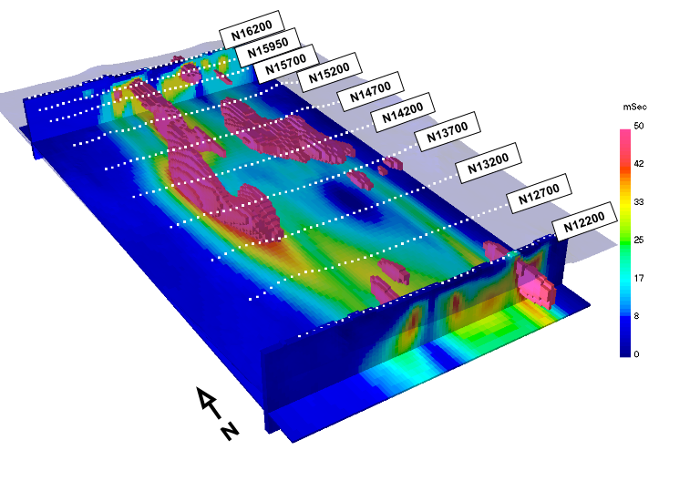
Fig. 451 3D conductivity obtained from 10 independent 2D inversions.
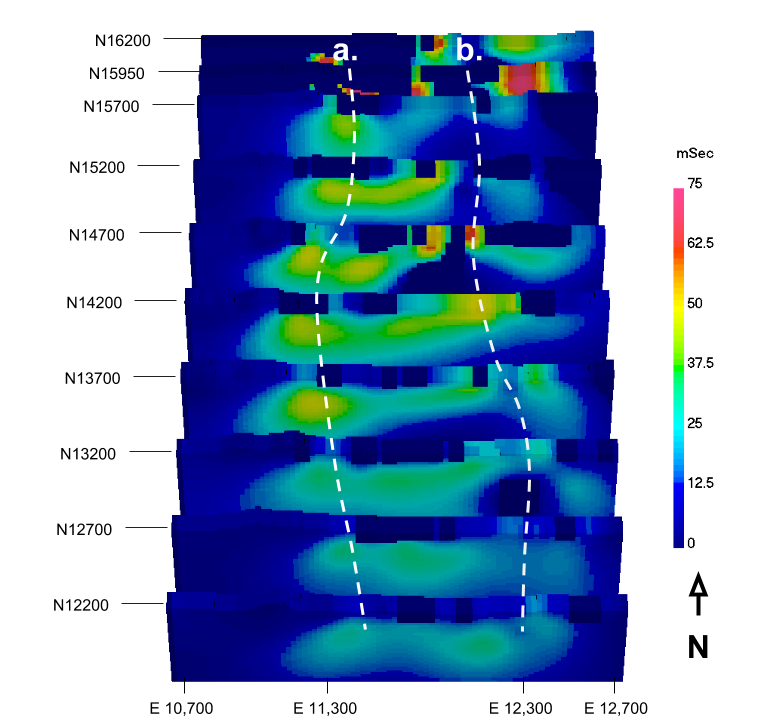
As a final step of data quality control, the P-DP and DP-P configurations are merged (Fig. 450) and re-inverted in 2D to attempt to recover a single distribution of conductivity. In preparation for the 3D inversion, the individual 2D models are transferred onto a 3D mesh shown in Fig. 451. Since each 2D model is the result of an independent inversion, small-scale discrepancies are to be expected. We note, however, several features are recovered on all 10 lines, supporting the idea of a strongly north-south oriented “2D” earth. The two main anomalies consistent throughout the inversions are:
A resistive domain on the western edge of the survey, marked by a steeply dipping contact near location 11,300 m, which may correspond to the Surprise Creek Formation
A narrow, steeply dipping conductor near 12,300 m, adjacent to a more resistive unit, possibly the conductive Breakaway Shale within a resistive Native Bee Siltstone.
Consistent 2D inversions in good agreement with the known geology increases our confidence in the data.
Table 15 : 2D inversions of combined P-DP and DP-P DCR data
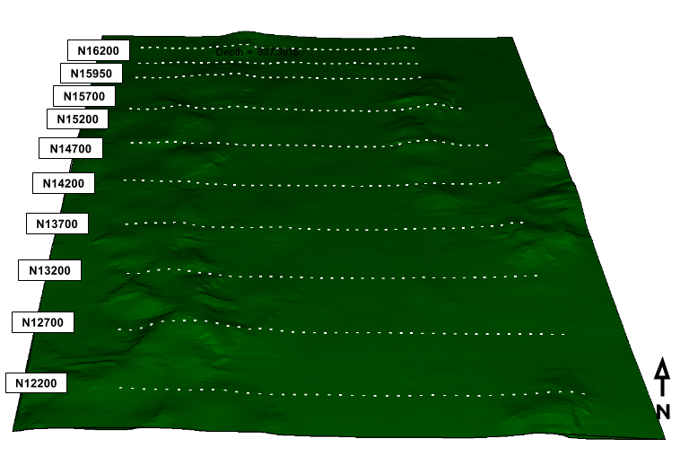
Fig. 452 : Perspective view of topography and electrode locations over the 3-D domain.
In preparation for the 3D inversion of the DCR data, locations were geo-referenced in planimetry to the local grid (Fig. 452). The vertical position of the electrodes were re-assigned based on a global DEM provided by Geoscience Australia to minimize topographic effects. A model mesh was constructed to discretize the subsurface into 25 x 50 x 15 m blocks. In total, 3678 P-DP and DP-P observations were inverted. Additional smoothing in the N-S orientation was applied in order to compensate for the 500-m line spacing. The initial inversion had 21 data outside a normalized misfit of 3, meaning that those predicted data were more than three times their uncertainties away from the observed data. They were removed and the data set was re-inverted.
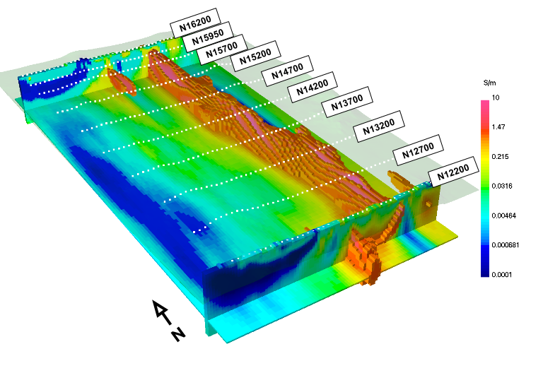
The 3D model can be viewed through the animation video that slices vertically and then horizontally through the model. The main feature is the large steeply conductor on the eastern side. The final portion of the animation shows the conductivity as an iso-surface, using a threshold that progressively increases in magnitude. The final image shows only cells that have a conductivity greater than 1 S/m. There is a moderate conductivity feature to the west of the large conductor as well as a smaller conductor near the south-east corner. These are illustrated in the single image presented in Fig. 453. Overall, the 3D inversion confirms that the geology over the Cluny region is mostly 2D, with alternating regions of high and low conductivity trending north-south indicating a steeply dipping geology.
Animation of the recovered 3-D conductivity model.
Fig. 453 : Sections through the recovered conductivity model and a volume rendered image of conductivities less than 1 S/m. The topographic surface and electrode locations (white dots) are shown for reference.
Our goal here is to generate a 3D subsurface chargeability model. 2D inversions are carried out for quality control purposes and to provide a first pass interpretation. The conductivity obtained from the 2D inversions above are used to generate sensitivities for the 2D IP inversions presented in the previous section.
As presented in the previous section, the MIMDAS system collects simultaneously a pole-dipole (P-DP) and a dipole-pole (DP-P) data configuration. Accordingly, the P-DP and DP-P data were inverted separately in 2D. As in the paper by Rutley et al, the uncertainties were assigned as 5% of the data amplitude with a minimum floor value of 2ms. The data are inverted, but the inversions struggled to reproduce the data and did not have any coherent model structure. The desired data misfit was increased by a factor of two. The data were re-inverted and the figure below shows the observed, predicted, and recovered models for both configurations and for each of the ten 2D lines. The increase of the desired misfit allowed more model regularization to produce a smoothly varying model with both the P-DP and DP-P configurations agreeing on the general distribution of chargeabilities.
Table 16 : Independent 2D inversions of the P-DP and DP-P IP data
As a final step of data quality control, the P-DP and DP-P configurations are re-merged and re-inverted in 2D to attempt to recover a single subsurface distribution of chargeability. In preparation for the 3D inversion, the individual 2D models are transferred onto a 3D mesh shown in Fig. 454. Since each 2D model is the result of an independent inversion, small-scale discrepancies are to be expected. We note, however, the sections vary smoothly from line to line.
Table 17 : 2D inversions of merged P-DP and DP-P IP data
In preparation for the 3D inversion of the IP data, locations were geo-
referenced in planimetry to the local grid (Fig. 452). The
vertical position of the electrodes were re-assigned based on a global DEM
provided by Geoscience Australia to minimize topographic effects. The model
mesh constructed for the 3D DCR inversion was used as well as the 3D recovered
conductivity model. In total, 3243 P-DP and DP-P observations were inverted.
Additional smoothing in the N-S orientation was applied in order to compensate
for the 500-m line spacing. The desired data misfit was set to two times the
number of data as with the 2D inversions. The 3D model can be viewed through
the animation video that slices vertically and then horizontally through the
model. The final portion of the animation shows the chargeability as an iso-
surface, using a threshold that progressively increases in magnitude. The
final image shows only cells that have a chargeability greater than 50 msec.
Sections through the recovered 3D chargeability model are presented in
Fig. 455. Overall, the IP inversion shows a complex region
of north-south trending chargeability in center of the volume but the linear
chargeability feature that coincides with the region of moderate conductivity
is of most interest.
Animation of the recovered 3-D chargeability model.
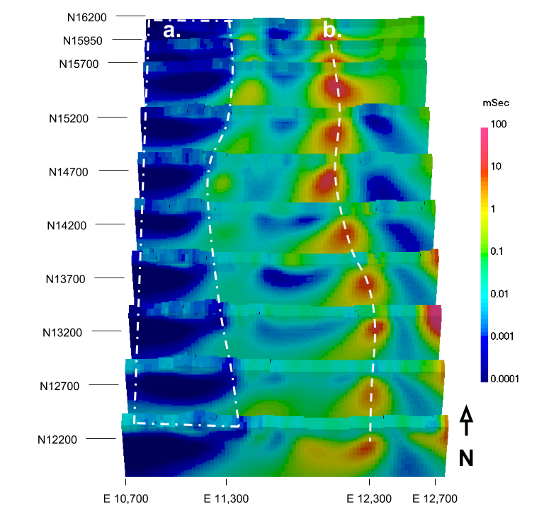
Fig. 455 Sections throughout the recovered chargeability model with a 3D volume
rendered image of chargeabilities higher than 50 msec. The topography
surface and electrode locations (white dots) are shown for reference.