Processing

In this step, we process the field data for the preparation of interpretation. Many different processing methods exist for airborne EM, but the-state-of-art is quantiative inversion that converts the measurements of EM fields to a conductivity model. In hydrological studies where the strata are almost horizontal, 1D layered earth modeling is usually the standard practice. In the following, we describe our processing in two steps: (1) data quality control and (2) 1D inversion.

Quality control of frequency domain data

Although the contractors have preliminarily processed the raw data to suppress the noise, there is still unwanted interference in the deliverables that can potentially harm the inversion. So our quality control precedure is supposed to prepare the data for inversion.

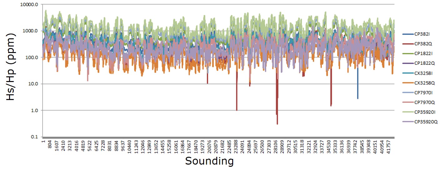
Fig. 354 Quality control of the FDEM data.

Viewing the plot of data for each frequqncy Fig. 354, we identify some unrealistically small outlies, and we decide to remove them from the data set. The uncertainty assigned to this data set is 5% plus 10 ppm as a floor.

Quality control of time domain data

For quality control, the SkyTEM data are also viewed for individual time channels along the flight lines Fig. 355. There are noticeable irregular data called “channel jumping”, and noise that contaminates the late time channels. The unrealistic decays and outlies can be automatically detected by the analysis of first or second derivative, and be removed. The noise present in the late times provides an estimate of a noise floor. The assigned uncertainty to the data is 10% plus 1E-13.

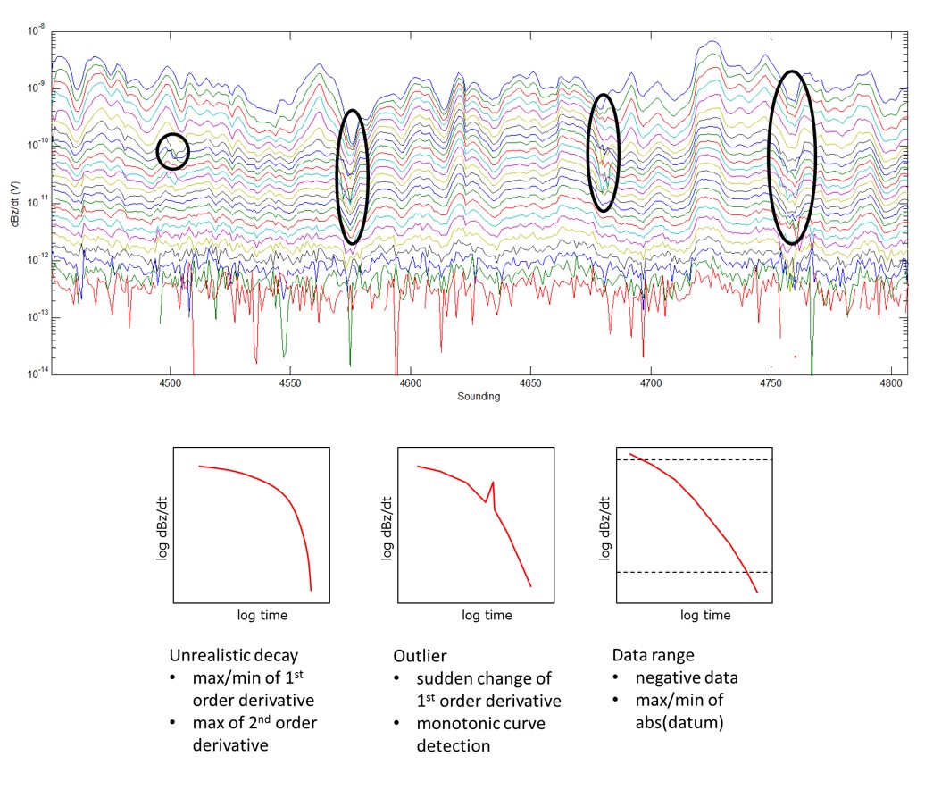
Fig. 355 Quality control of the TDEM data.

1D layered earth inversion

The two data sets in this case history have been previously inverted using spatially constrained inversion by [VAM09]. Here we present the inversion results obtained using UBC-GIF programs.

Layered model

A layered model treats the earth below the surface as a stack of horizontally infinite layers, each of which has a constant conductivity value. In our precedure, every sounding is given a layered model, and the conductivity values of the layers are sought by the inversion with the observed data at that sounding. The output of each sounding inversion is a series of conductivity values as a function of depth. Finally, all the 1D functions of conductivity at different locations are stitched together to form a 3D volume.

For consistency, both the FDEM and TDEM inversion share the same layer thicknesses. Because the smallest skin depth or diffusion distance is about a couple of meters, we design the top layer to be 1 m thick. The thickness increases geometrically from the surface to the depth of 225 m. There are 21 layers in total.

Inversion result

Inversions of the TDEM and FDEM data sets are carried out on a sounding-by- sounding basis. Most soundings achieve the desired misfit except that some soundings fail to converge due to excessive noise or coherent bias in the data. Fig. 356 shows the depth slices of the stitched volume of conductivity from the FDEM and TDEM inversions. Although the data maps of the two data sets are in different units and have different apparence, the reconstructed conductivity models are highly consistent. This demonstrates the necessity of inversion-based processing and interpretation.

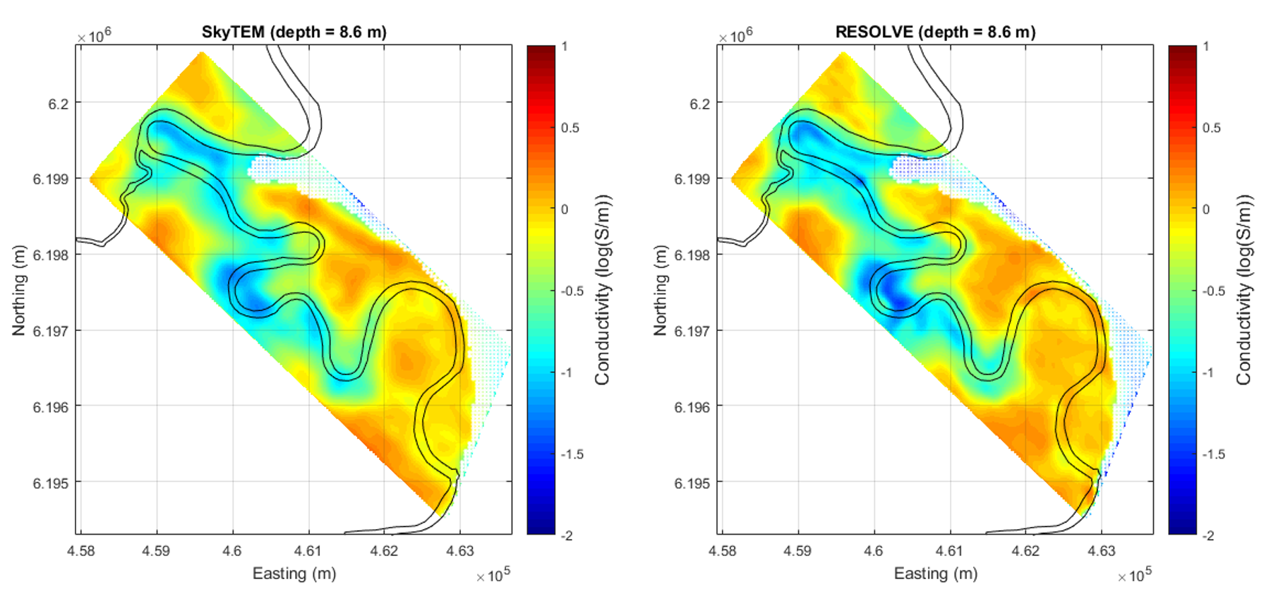
Fig. 356 Inversion models of the TDEM and FDEM data sets at Bookpurnong. The shaded area indicates the highland where irrigation takes place.