Processing

The field data were provided in units of pV/(Am^4), meaning the data are normalized by the current (A) in the transmitter, the area (m^2) of the transmitter, and the area (m^2) of the receiver. In order for us to work with these data, we first change them so the units are V/(Am^2). This assumes that the receiver is at a point location rather than being defined as a loop with a certain area. For the VTEM system used in 2014, the transmitter had a radius of 13 m. The transmitter area was multiplied by the data to get the data in the desired units.

Our goal is to obtain a 3D model of the subsurface to understand how the resistivity changes with depth and in the northing and easting directions. Before actually working with the field time-domain data, we use a synthetic model is to better understand the data and determine what parameters should be used in the inversion.

1D inversion of synthetic data

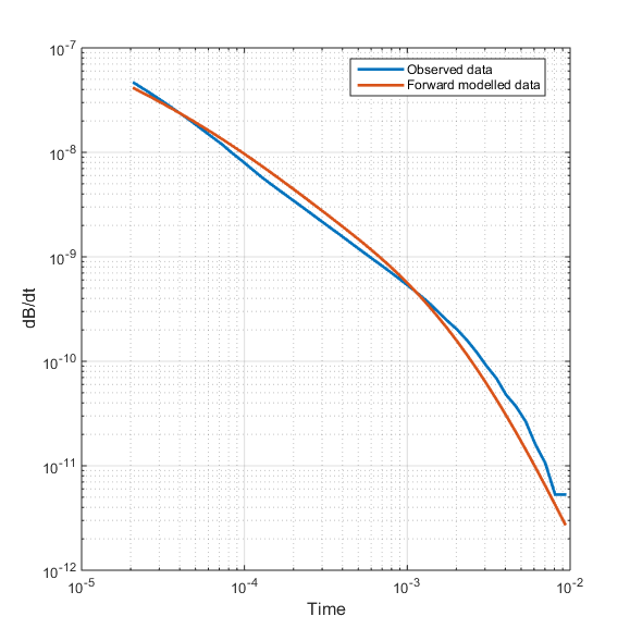
Fig. 298 The blue line shows a randomly-chosen decay curve from the VTEM field data set. The orange line is the forward modeled data using the synthetic 1D model (shown in Fig. 292) from borehole data [DO16a]. The two decay curves are fairly similar to each other, suggesting that the 1D synthetic model is a decent representation of the resistivity structures at the Aspen property.

A one-dimensional model is a fair start to recovering information about the bavkground geology in the Athabasca oil sands as the different formations are generally flat-lying. The synthetic model developed from resistivity logging data thus provides a good starting point to forward model and invert airborne time-domain data.

A random sounding location is chosen from the VTEM data set and the transmitter and receiver parameters are used to forward model data using the synthetic 1D model (Fig. 292). The forward modeled data is compared to the actual field data in Fig. 298 and shows that the data fitting is good. This suggests that the synthetic model is a good representative of the resistivity structure at Aspen.

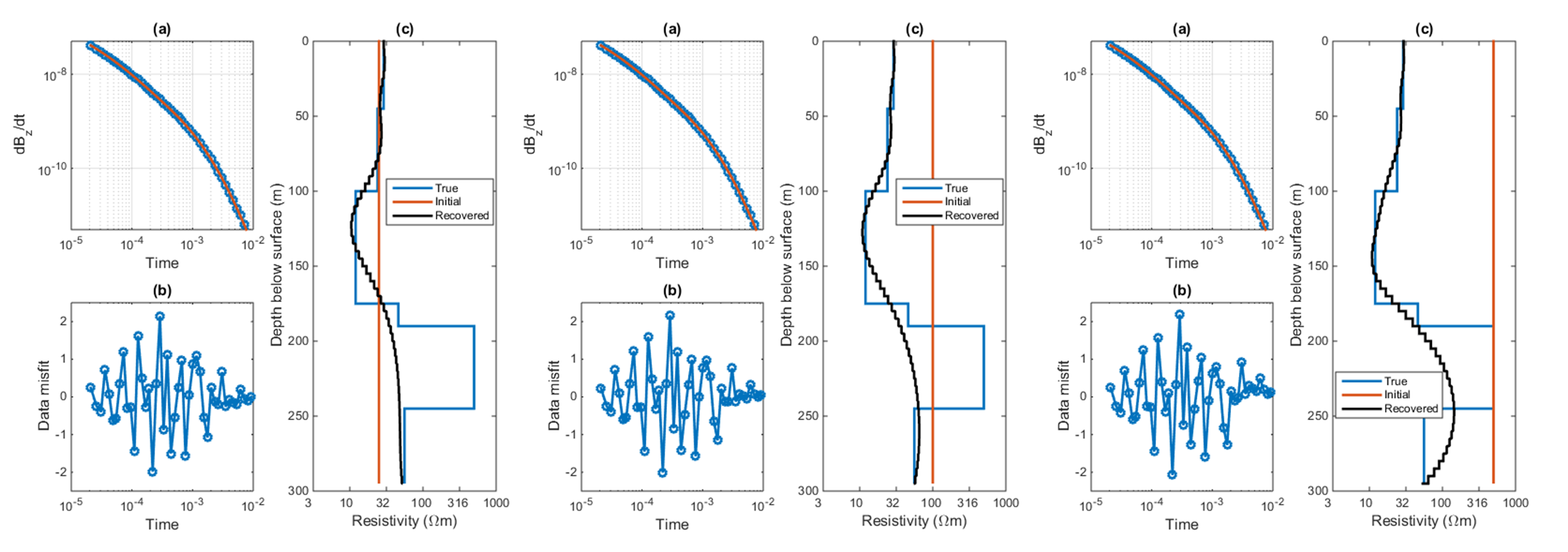
Gaussian noise of 1.5% is added to the forward modeled data and uncertainties are assigned as a percentage of the data and a noise floor: 1.5% and 1e-12 V. The synthetic decay curve is inverted using L2 norms for both the data misfit and the model objective function using UBC-GIF’s EM1DTM code [FO93]. Values for \(\alpha_s\) and \(\alpha_z\) are set to 0.001 and 1, respectively. An initial and reference model of 25 \(\Omega m\) was used. The results are shown in Fig. 299 (left). The predicted data fits the observed data very well and the data misfit is randomly distributed. The model recovers the layers up to a depth of approximately 175 m. Below 175 m, the data may have some sensitivity to the resistive McMurray Formation but this layer is not well-recovered in the inversion. To better understand the sensitivity of the data to layers at depth, the inversion is repeated using an initial and reference model of 100 \(\Omega m\). The results are shown in Fig. 299 (centre). The data are fitted just as well as in the previous inversion but the model slightly changes below 175 m. It is pushed closer to the initial/reference model, suggesting limited sensitivity to layers below the Clearwater Formation. This is further supported by a third inversion where the initial and reference model are set to 500 \(\Omega m\). The recovered model is shown in Fig. 299 (right).

Fig. 299 Inversion of the forward modeled data (Fig. 298) using an initial and reference model of (left) 25 \(\Omega m\), (centre) 100 \(\Omega m\), and (right) 500 \(\Omega m\). Below the conductive layer, the model pushes towards the reference model, providing an idea of the depth of investigation using the VTEM system for the Athabasca oil sands region. In each panel, (a) compares the observed (blue) and predicted (orange) data while (b) shows the normalized data misfit for each time channel. The recovered model (black) is shown in sub-panel (c) along with the true model (blue) and the initial/reference model (orange).

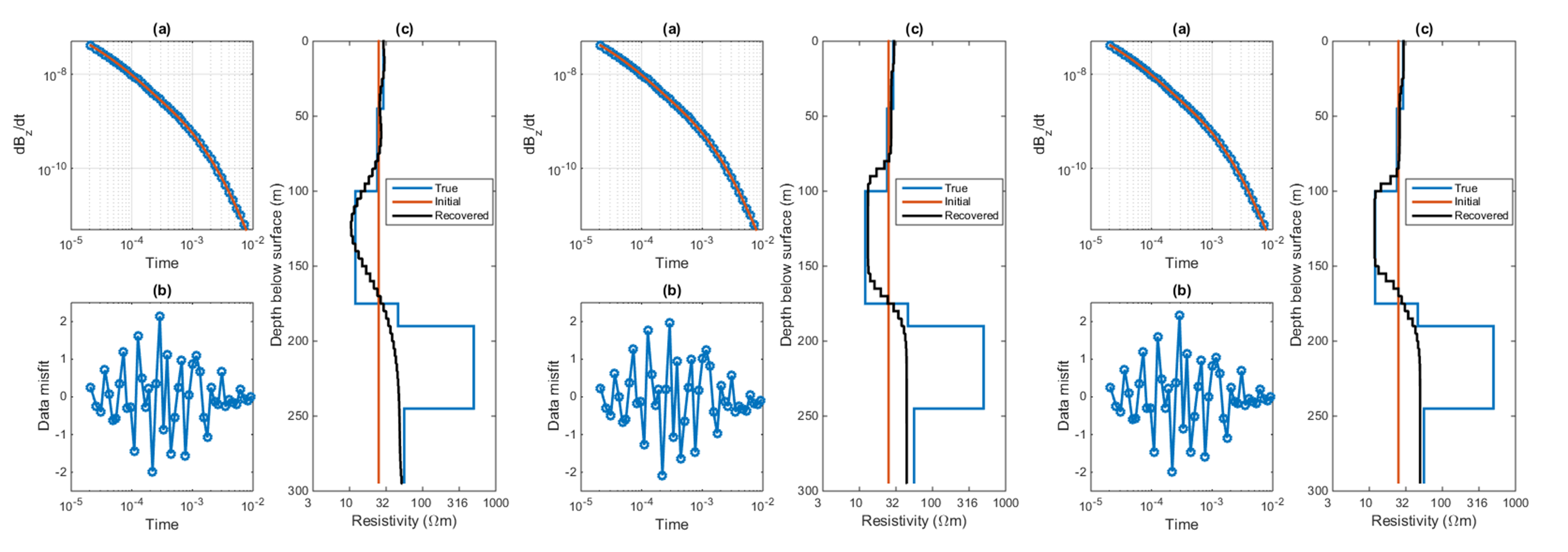
The synthetic decay curve is also inverted using an L1 norm for the model objective function (Equation ref{intro:phim}) to recover blockier models compared to the L2 norm. As the layers within the Athabasca oil sands tend to be well-defined, distinct units, using an L1 norm may allow for improved recovered models. The result is shown in Fig. 300 (centre) with the L2 results duplicated in Fig. 300 (left). The result is noticeably blockier, with better recovery of the Clearwater Formation. To generate an even blockier result, the value of \(\alpha_z\) is decreased from 1 to 0.1 to lessen smoothing on changes in the model. This result is shown in Fig. 300 (right). In all results, the observed data are reproduced well by the model and the normalized data fitting misfit is random. By decreasing \(\alpha_z\), the model is blockier compared to using the L1 norm alone.

Fig. 300 Inversion of the forward modeled data (Fig. 298) using an (left) L2 norm and (centre) L1 norm for $phi_m$. In (right), an L1 norm is used and \(\alpha_z\) is reduced from 1 to 0.1. In each panel, (a) compares the observed (blue) and predicted (orange) data while (b) shows the normalized data misfit for each time channel. The recovered model (black) is shown in sub-panel (c) along with the true model (blue) and the initial/reference model (orange).

The 1D inversions of the forward modeled data provide initial information about depth of investigation, the influence of inversion parameters, and what to expect in the recovered model. These parameters can be carried over to the inversion of field data using a pseudo-3D approach.

Regional pseudo-3D inversions of field data

To obtain a pseudo-3D model, 5,772 soundings are cooperatively inverted in 1D and interpolate the individual 1D models [FHC+14]. The 3D model has cells that extend 200 m in the easting and northing directions and 5 m in the vertical direction, allowing detailed information about the subsurface layers to be recovered. This method is appropriate for this region as the 1D assumption holds fairly well, given the expected layered geology at the Aspen property. An initial model of 25 \(\Omega m\) was used. For each inversion iteration, the reference model is updated to include the influence of nearby soundings. This gives a large-scale regional resistivity model.

The recovered model is interpreted using known geologic information about the area on the following page.