Data

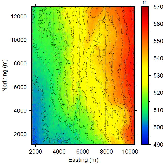
Fig. 295 Topography for the Aspen survey region.

In preparation for processing and inversion of the time-domain EM data, we first assess the data through visualization. The topography is shown in Fig. 295, showing higher elevations in the eastern part of the survey region. The elevation decreases towards the west.

The data consists of \(\partial \mathbf{B}/\partial t\) measurements at 44 time channels. A selection of time channel maps are shown in Fig. 296. We can associate higher values (warm colours) with conductive regions and lower values (cool colours) with resistive regions. The earliest times are fairly uniform and appear to be quite conductive. Middle time channels show more varying structures. The data decay as time goes on. This is much more apparent when plotting the data as decay curves.

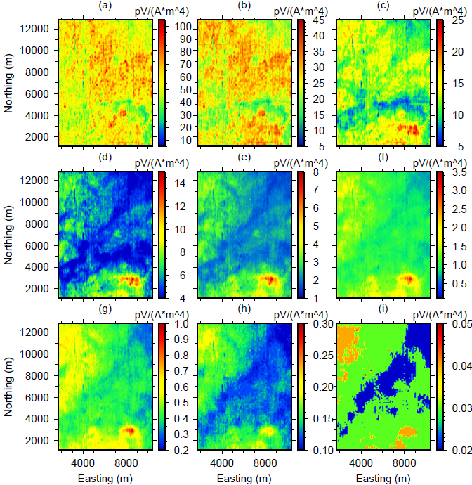
Fig. 296 Time channel maps showing \(\partial \mathbf{B}/\partial t\) for (a) 0.02, (b) 0.05, (c) 0.1, (d)0.19, (e) 0.33, (f) 0.77, (g 1.53, (h) 3.06, and (i) 9.29 millaseconds.

A selection of six decay curves are plotted in Fig. 297. Depending on their location in space, the decay curves show different characteristics. This gives us insight into the resistivity structures at those locations. Decay over conductive features is slower than over resistive features. Thus, we can deduce that the subsurface at Location 1 is more conductive than at the other locations. At middle times, Location 4 becomes more resistive compared to the other locations. When comparing to the time maps in Fig. 296, that region is more resistive than the surroundings. At later times, the decay curves are much more similar, suggesting less variations in the resistivity at depth. Both ways of plotting the data provides initial understanding of the data and the resistivity structures in the region.

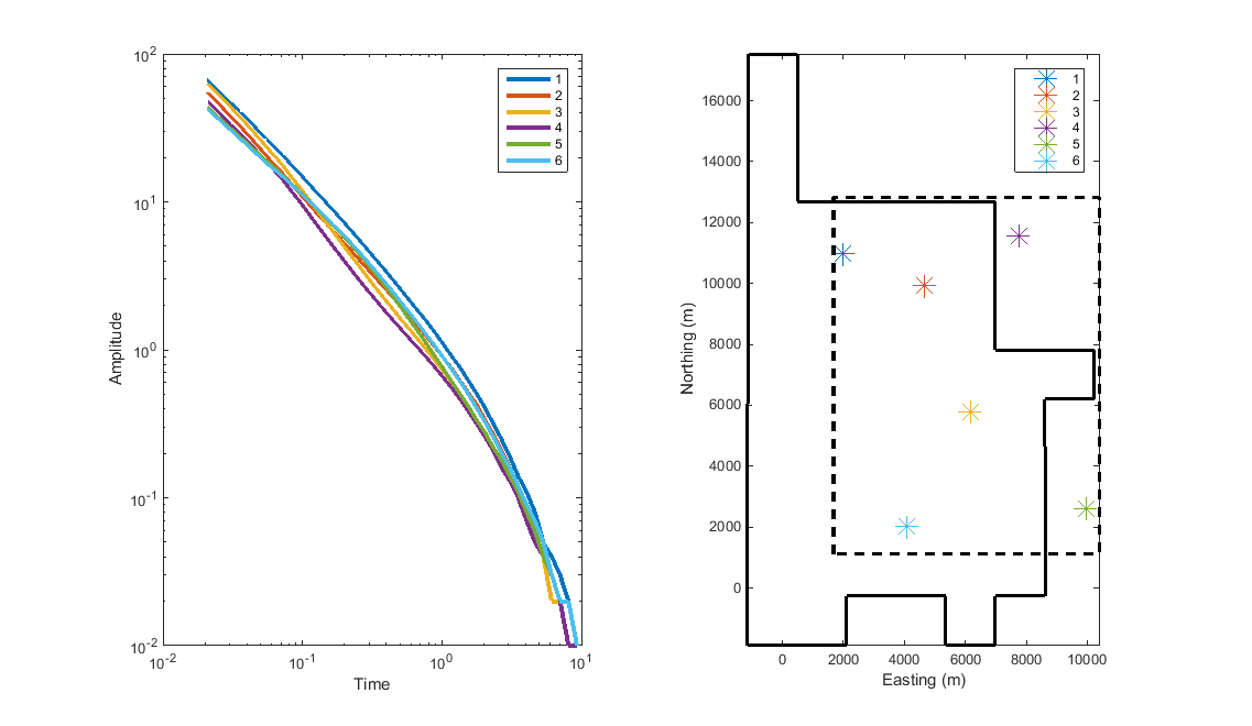
Fig. 297 The left panel shows 6 decay curves and the right panel shows their location with respect to the survey boundary (black, dashed) and the Aspen property boundary (black, solid).

We now turn our attention to processing the data to better understand what kind of information we can glean and how best to invert the data.