Intepretation

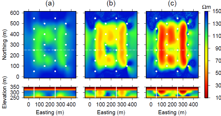
Fig. 492 Results from cascading time-lapse inversion for (a) early time, (b) middle time, and (c) late time.

The recovered models for each time step are shown in Fig. 492. Because this is a synthetic example, Fig. 493 shows the true models at each time step. The first major observation is that the horizontal locations of the steam chambers are well-imaged at each time step. The vertical resolution is less desirable but still shows that the steam chambers grow vertically and expand into the reservoir. If required, the vertical resolution could be improved by increasing the number of receivers within the reservoir.

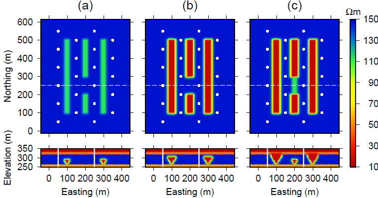
Fig. 493 True models at three time steps: (a) early time where the chambers are 20 m high and 11 m at their widest, (b) middle time where the chambers are 35 m high and 20 m at their widest, and (c) late time where the chambers are 50 m high and 28 m at their widest. In (c), steam has penetrated through a blockage shown in (a) and (b) and grown to a height of 20 m and width of 11 m. Each panel shows a depth slice 215 m below the surface and a cross-section of the reservoir at a northing of 250 m. In plan view, white dots denote borehole locations and the white line indicates the location of the cross-section. The borehole locations in the cross-sections are indicated using white dots.

In addition, the EM method is capable of imaging the gap in the middle steam chamber, where steam is being blocked, possibly due to heterogeneity within the reservoir. This result can provide critical information to production engineers since a gap in the middle conductive chamber indicates that no steam is penetrating and thus no oil is being produced.

Att the last time step, some growth occurs in the center of the middle steam chamber and this is reflected in the recovered model. This again shows that the survey is sensitive to these resistivity changes and has enough resolution to recover those changes using inversion.