Data and Processing

Surface-Based GPR Surveys

The processing sequence applied to the surface-based GPR data is relatively standard (Table 4). An example of applying this sequence to profile G2 is presented in Fig. 413. Although the G2 image is relatively noisy with numerous artifacts, some clear dipping events are seen between 500 and 1100 ns. Do these represent subsurface reflections? Unfortunately, comparable events are not observed on the G1 and G3 images, long portions of which are practically coincident with or only a few meters from the G2 image (compare images in Fig. 414).

The 25 MHz image in Fig. 414 c helps explain the inconsistencies between coincident and adjacent GPR sections. We interpret the mostly curvilinear events in the top 500 ns of Fig. 414 d as in plane and out of plane diffractions generated at the boundaries between the snow cover and rugged bouldery surface and at buried boulders. Recording 25 MHz GPR data along a second profile offset by only a few meters would result in comparably complex diffraction patterns, but it would be nearly impossible to correlate events on the two profiles. Accordingly, we conclude that the primary explanation for inconsistent surface-based GPR images is the overwhelming effects of in plane and out of plane diffractions.

Table 4: Processing scheme applied to the surface-based GPR data collected across the Furggwanghorn rock glacier.

Step	Details
Coordinate assignment to traces	Coordinates from differential GPS
Time-zero corrections	Manual pick of direct wave
Removal of high amplitude first arrivals
Automatic gain control	100 ns
Moving singular value decomposition filter (only applied to pulseEKKO data)	20-trace window largest 2% eigenvalues set to 0
Bandpass filter	10 - 110 MHz (50MHz); 3 - 60 MHz (25MHz)
Binning	Bin size 0.5-0.8m depending on original trace spacing
Moving average filter	Weighted average of 3 traces
Trace equalisation	Equalisation of the mean amplitudes
Kirchhoff time migration	Constant velocity 0.13 m/ns
Elevation corrections	Simple elevation static corrections
Time-depth conversion	Same velocity model as for the migration

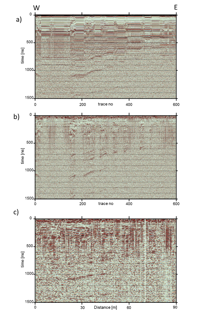
Fig. 413 Example of the processing sequence in Table 4 applied to surface-based GPR profile G2. (a) Raw data after time zero correction and automatic gain control. (b) As for (a) after application of a singular value decomposition filter and bandpass filter. (c) As for (b) after trace binning, application of a moving average filter and trace equalization. V : H ≈ 1 : 2.

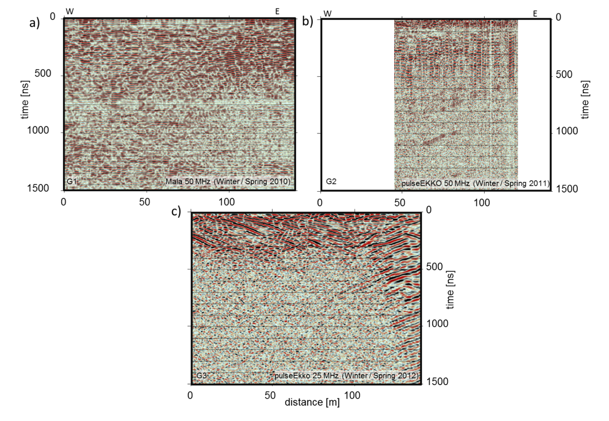
Fig. 414 Comparison of nonmigrated sections acquired at the same general location along similarly oriented profiles (see caption to Fig. 412 for locations) using the different surface-based GPR systems shown in Fig. 412 a ‑ c: (a) 50 MHz Mala Rough Terrain Antennae, (b) 50 MHz pulseEKKO PRO (same section as shown in Fig. 413 c, but with different vertical and horizontal scaling for better comparison with the other sections), (c) 25 MHz pulseEKKO PRO. V : H ≈ 1 : 1.

H-GPR Surveys

Strong horizontal noise dominated the raw H-GPR data (Fig. 415 a). Fortunately, this noise, which was generated by the helicopter, was sufficiently coherent and predictable that it could be eliminated and the geological signal enhanced by applying carefully designed singular value decomposition filters, appropriate gain functions and F-X deconvolution (Table 5; Fig. 415 b). The processed data were Kirchhoff time migrated (Fig. 415 c) and converted to depth using a simple ground velocity model. Unlike the surface-based GPR examples, the H-GPR images are consistent from line to line and from year to year (Fig. 416 and Fig. 417). [MMR+16] argue that the superiority of the H-GPR images relative to the ground-based ones is not related to the different GPR instruments that were employed. Instead, they suggest that the H-GPR images are affected by much weaker near surface diffractions and that there is only insignificant coupling between the H-GPR antennae and the snow and near surface heterogeneities.

Table 5: Processing scheme applied to the H-GPR data collected across the Furggwanghorn rock glacier.

Step	Details
Coordinate assignment to traces	Coordinates from differential GPS
Moving singular value decomposition filter	100-trace window, largest 2% eigenvalues set to 0
Inverse average envelope gain	Envelope derived from the reflection strength
F-X deconvolution	40 - 180 MHz, horizontal window length 50 traces, time window length 100ns, overlap 50 ns
Trace equalisation	Equalisation of the mean amplitudes
Kirchhoff time migration	Constant velocities of 0.13 and 0.30 m/ns for the ground and air, respectively
Elevation corrections	Elevations based on a digital elevation model
Time-depth conversion	Same velocity model as for the migration

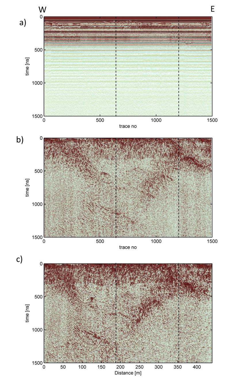
Fig. 415 Example of the processing sequence in Table 5 applied to H-GPR data recorded along profile H5 in Fig. 412. (a) Raw data after removal of system gain. (b) As for (a) after application of a singular value decomposition filter and gain function, F-X deconvolution and trace equalisation. (c) As for (b) after Kirchhoff time migration. An air layer has been removed (i.e. reflections from the surface appear at time equals zero). V : H ≈ 2.8 : 1.0.

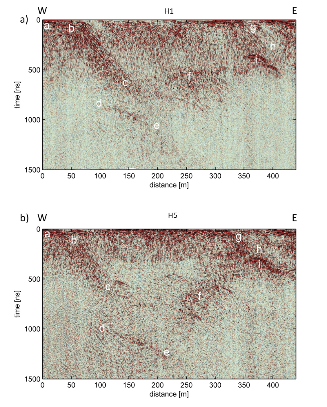
Fig. 416 Comparison of nearly coincident (a) H1 and (b) H5 nonmigrated H-GPR sections, which were recorded in Winter / Spring 2012 and Winter / Spring 2013, respectively (see Fig. 412 for locations). Letters a ‑ i identify distinct features and patterns observed in both sections. An air layer has been removed (i.e. reflections from the surface appear at zero time). V : H ≈ 2.8 : 1.0.

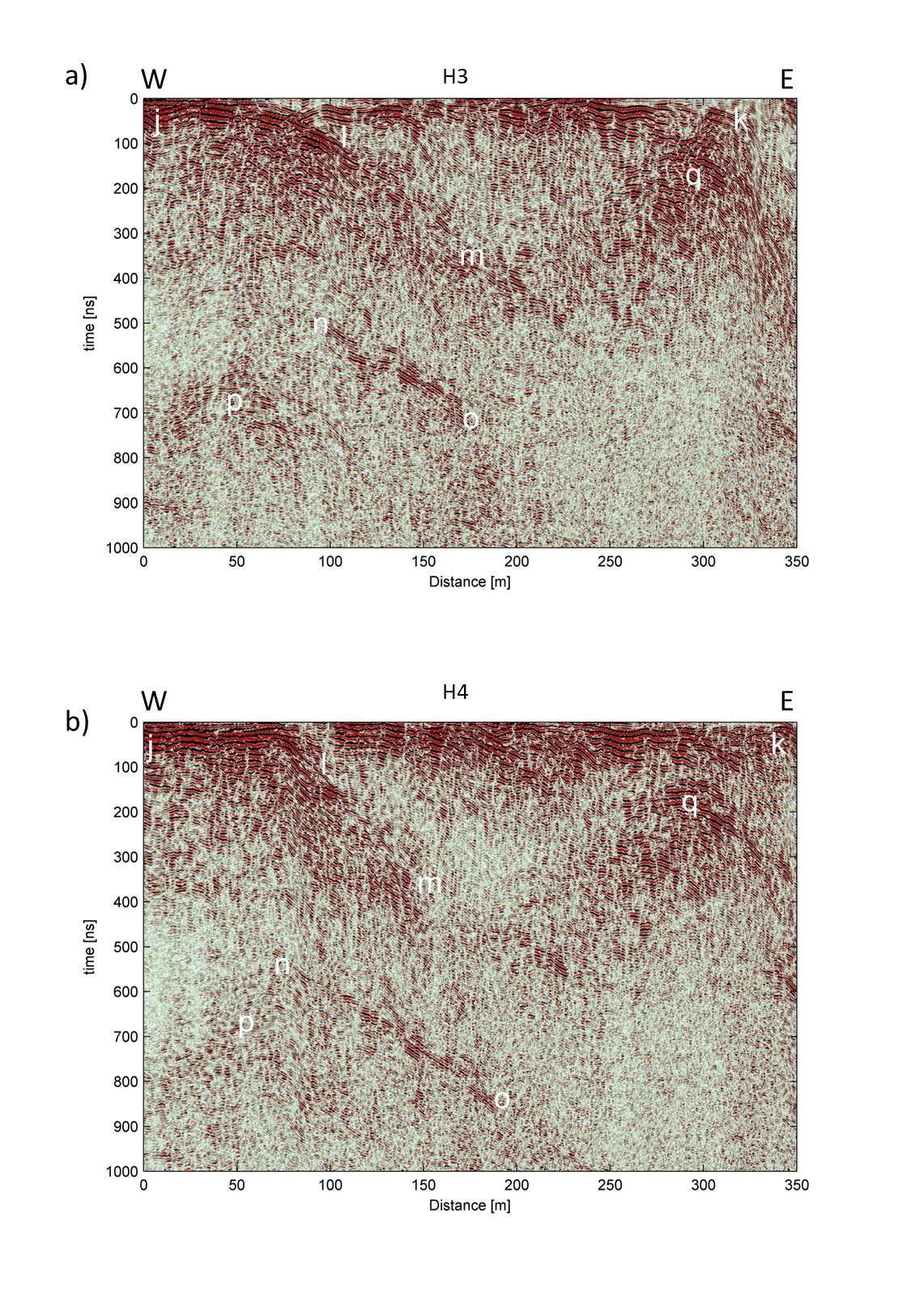
Fig. 417 Comparison between nearly parallel (a) H3 and (b) H4 nonmigrated H-GPR sections, both of which were recorded in Winter / Spring 2013 (see Fig. 412 for locations). Letters j - q identify distinct features and patterns observed in both sections. An air layer has been removed (i.e. reflections from the surface appear at zero time). V : H ≈ 3.5 : 1.0.