Impulse Response

Purpose

The sphere’s time-dependent response to an arbitrary excitation is represented by its impulse response. Here, analytic expressions for the sphere’s impulse response are presented for a permeable and a non-permeable sphere.

Introduction

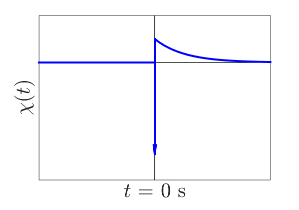
Fig. 142 Representation of the impulse response for the excitation of a conductive and permeable sphere.

According to our general formulation, the induced dipole moment \(m(t)\) characterizing the sphere is defined by a convolution:

(452)\[m(t) = \Bigg ( \frac{4\pi}{3} R^3 \Bigg ) \int_{-\infty}^\infty \chi (\tau) h_0 (t-\tau )d\tau\]

where \(R\) is the sphere’s radius, \(\chi (t)\) represents the sphere’s impulse response and \(h_0 (t)\) represents the inducing field. By definition, \(\chi (t)\) is the inverse Fourier transform of the sphere’s frequency-dependent excitation factor ([Wai51]):

(453)\[\chi (t) = \frac{1}{2\pi} \int_{-\infty}^{\infty} \chi (i \omega) e^{i\omega t} d\omega\]

The general shape of the impulse response for a conductive and magnetically permeable sphere is shown in Fig. 142. At \(t<0\), the impulse response is zero. This indicates that the sphere’s TEM response is causal. As a result, an convolution with the sphere’s impulse response can be expressed as an integral from 0 to \(\infty\):

\[\chi (t) \otimes g (t) = \int_0^\infty \chi (\tau) g (t-\tau) d\tau\]

Ultimately, the sphere’s TEM response depends on the scaling of the delta function which occurs at \(t=0\) and the decay which is observed for \(t>0\). Below, analytic expressions for the impulse response for permeable and non-permeable sphere’s are presented. Derivations used to obtain these expressions are found in the following section.

Conductive Sphere

For a conductive and non-permeable (\(\mu = \mu_0\)) sphere, the impulse response is given by ([WS69]):

(454)\[\chi (t) = - \; \frac{3}{2} \delta (t) - \frac{9}{2} \Bigg [ \frac{1}{\beta^2} - \frac{1}{\beta \sqrt{\pi t}} \Bigg ( 1 + 2 \sum_{n = 1}^\infty e^{-(n\beta)^2/t} \Bigg ) \Bigg ] u(t)\]

where \(\delta (t)\) is the Dirac delta function, \(u(t)\) is the unit-step function and:

(455)\[\beta = (\mu_0 \sigma )^{1/2} R\]

Conductive and Permeable Sphere

For a conductive and permeable sphere, the impulse response is given by ([WS69]):

(456)\[\chi (t) = - \, \frac{3}{2} \delta (t) + \, \frac{3}{2} \Bigg ( \frac{6 \mu_r}{\beta^2} \sum_{n=1}^\infty \frac{ \xi_n^2 \, e^{-\xi_n^2 t/\beta^2}}{(\mu_r + 2)(\mu_r - 1)+\xi_n^2} \Bigg ) u(t)\]

where:

\[\beta = (\mu \sigma )^{1/2} R\]

Coefficients \(\xi_n\) within the sum are defined by:

\[\textrm{tan} \, \xi_n = \frac{(\mu_r - 1)\xi_n}{\mu_r - 1 + \xi_n^2}\]

From Wait and Spies ([WS69]), coefficients \(\xi_n\) are spaced roughly \(\pi\) apart with:

\[n\pi \leq \xi_n \leq (n+1/2) \pi\]

The value of each coefficient may be found iteratively using very few iterations (< 10) according to:

\[\xi_n^{(k+1)} = n\pi + \textrm{tan}^{-1}\Bigg ( \frac{(\mu_r - 1) \xi_n^{(k)}}{\mu_r - 1 + (\xi_n^{(k)} )^2} \Bigg )\]