Excitation Factor for Special Cases

Purpose

The characteristic dipole response from a conductive and magnetically permeable sphere is defined by its excitation factor. Here, we present analytic expressions and discuss the excitation factors for several specific cases, including: a conductive and magnetically permeable sphere, a purely conductive sphere, and the zero-frequency response from a highly permeable sphere.

Conductive and Magnetically Permeable Sphere

According to Wait ([Wai51]), the excitation factor for a conductive and magnetically permeable sphere is given by:

(386)\[\chi (i \omega) = \frac{3}{2} \Bigg [ \! \frac{2\mu \big [ tanh(\alpha) - \alpha \big ] + \mu_0 \big [\alpha^2 \, tanh(\alpha) - \alpha + tanh(\alpha) \big ] }{\mu \big [ tanh(\alpha) - \alpha \big ] - \mu_0 [ \alpha^2 \, tanh(\alpha) - \alpha + tanh(\alpha) \big ] } \! \Bigg ]\]

where

\[\alpha = \Big [ i\omega\mu\sigma \Big ]^{1/2}R\]

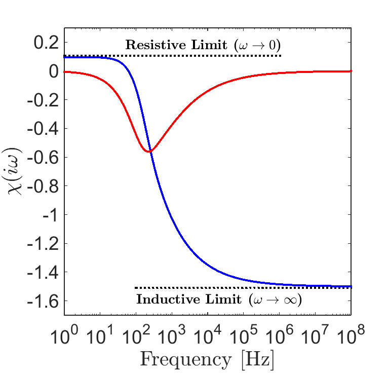
Fig. 123 Excitation factor for a conductive and magnetically permeable sphere in free-space with \(R\) = 25 m, \(\sigma\) = 10 S/m, and \(\mu\) = 1.1 \(\mu_0\).

The excitation factor for a sphere with \(R\) = 25 m, \(\sigma\) = 10 S/m and \(\mu\) = 1.1 \(\mu_0\), can be seen in Fig. 123. At low frequencies, \(\chi (i\omega)\) is positive, implying the excitation of the sphere is parallel to the inducing field. Because the EM induction is negligible at sufficiently low frequencies, this case represents a purely magnetic response by the sphere. At high frequencies, \(\chi(i\omega)\) is negative. Therefore, inductive excitation of the sphere will oppose the inducing field. The inductive and resistive limits of the excitation factor can be obtained by taking the limits of Eq. (386):

(387)\[\begin{split}\chi (i\omega) = \begin{cases} \dfrac{3 \big ( \mu - \mu_0 \big )}{ \big ( \mu + 2 \mu_0 \big ) } & \textrm{ as } \omega \rightarrow 0 \\ \\ - \dfrac{3}{2} & \textrm{ as } \omega \rightarrow \infty \end{cases}\end{split}\]

Thus regardless of the sphere’s physical properties, the inductive limit of the sphere’s excitation factor is the same, whereas at the resistive limit, it depends on the sphere’s magnetic properties.

Purely Conductive Sphere

For a purely conductive object (i.e. \(\mu = \mu_0\)), Eq. (386) can simplified to the following:

(388)\[\chi (\omega) = - \; \frac{3}{2} \Bigg [ 1 + \frac{3}{\alpha^2} - \frac{3 \, \textrm{coth}(\alpha)}{\alpha} \Bigg ]\]

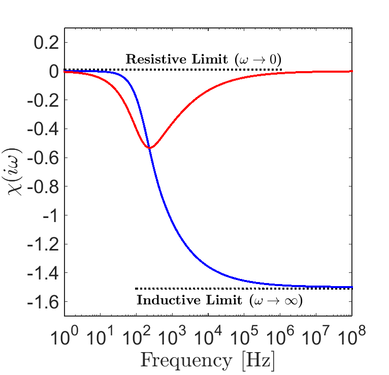
Fig. 124 Excitation factor for a conductive sphere in free-space with \(R\) = 25 m, \(\sigma\) = 10 S/m, and \(\mu\) = \(\mu_0\).

The excitation factor for a sphere with \(R\) = 25 m, \(\sigma\) = 10 S/m and \(\mu\) = \(\mu_0\), can be seen in Fig. 124. Because the sphere is non-permeable, there is no magnetic response at low frequencies. Thus we expect \(\chi (i\omega) \rightarrow 0\) as \(\omega \rightarrow 0\). At higher frequencies however, the sphere’s inductive response is approximately equal to that of the previous case. This can be shown by taking the inductive and resistive limits of Eq. (388):

(389)\[\begin{split}\chi (i\omega) = \begin{cases} \; \; 0 & \textrm{ as } \omega \rightarrow 0 \\ \\ -\dfrac{3}{2} & \textrm{ as } \omega \rightarrow \infty \end{cases}\end{split}\]

Therefore, a purely conductive sphere will only experience excitations which oppose the inducing field.

Low-Frequency Limit for Highly Permeable Spheres

The excitation factor for a highly permeable sphere at low frequency can be obtained by examining the resistive limit of Eq. (386). Where \(\kappa\) is the magnetic susceptibility (link) of the sphere, and \(\mu =\mu_0 \big [ 1 + \kappa \big ]\):

(390)\[\lim_{\omega \rightarrow 0} \; \chi (i\omega) = \dfrac{3 \big ( \mu - \mu_0 \big )}{ \big ( \mu + 2 \mu_0 \big ) } = \dfrac{3 \kappa }{3 + \kappa} = \bar \chi (\kappa)\]

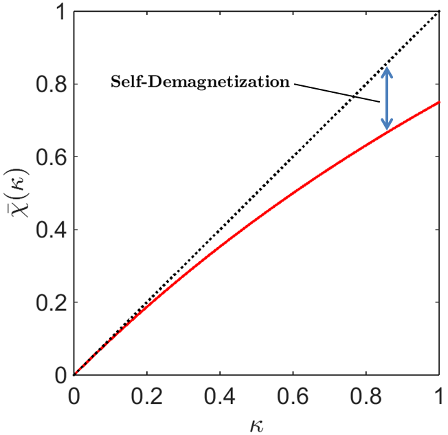
Fig. 125 Zero-frequency excitation facter at \(\omega\) = 0 for increasing magnetic susceptibilities (red), compared to a linear trend with respect to \(\kappa\) (black).

\(\bar \chi (\kappa)\) represents the zero-frequency excitation factor for a permeable sphere, and depends on the sphere’s magnetic susceptibility. The zero-frequency excitation factor \(\bar \chi (\kappa)\), as a function of \(\kappa\) is plotted in Fig. 125.

For small magnetic susceptibilities (\(\kappa < 0.1\)), the relationship between \(\kappa\) and the excitation factor is approximately linear. For large values however, the effects of self-demagnetization (link) within the sphere will result in a proportionally weaker induced dipole moment. The effects of self-demagnetization for the sphere are given by:

(391)\[\textrm{S. D.} = \kappa - \bar \chi (\kappa) = \frac{\kappa^2}{3 + \kappa}\]

The largest possible magnetic response from a sphere can be obtained by taking the limit of Eq. (387) as \(\kappa \rightarrow \infty\):

(392)\[\lim_{\kappa \rightarrow \infty} \, \bar \chi (\kappa) = 3.\]