Circuit Model for EM Induction
Purpose
The basic principles for EM induction were outlined in Link. Here we use an equivalent electric circuit model consisting of three loops to represent that process. We derive the inductive response function in terms of circuits, mutual and self-inductance, and coupling. Widgets are developed to help physical understanding. The response functions for many practical geophysical surveys resemble that from the circuit model and hence much intuition about EM signals can be obtained using this analysis.
The basic EM survey is shown in Fig. 89. The time varying magnetic field (referred to as the primary field) in the Tx induces currents in the conductor. Those currents produce a secondary field that can be recorded at the receiver.
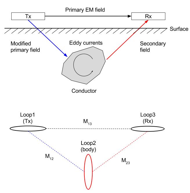
Fig. 89 Conceptual diagrams for EM inductions. Top panel shows excitation of the conductor using induction, and botton panel shows corresponding 3-loops system.
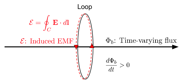
From Faraday’s Law, we establish the link between EMF (\(\mathcal{E}\), voltage), and time varying flux (\(\Phi_b\)). Below diagram illustrates how EMF could be generated from time-varying flux (\(\mathcal{E}= - \frac{d \Phi_b}{dt} = \imath \omega \Phi_b\)). The EMF (voltage) produces a current in the loop.
The circuit model is now understood as follows:
Loop 1: is the transmitter (Tx). It has a time varying current (I1 e^iwt) and hence produces a time varying field everywhere in space.
Loop 2: represents the conductive body. The time varying flux generates currents in the conductor (\(I_2 e^{\imath \omega t}\)). These time varying currents produce a time varying field everywhere in space.
Loop 3: is the receiver (Rx). The measured EMF, \(\mathcal{E}^t\) is
\[\mathcal{E}^t = \mathcal{E}^p +\mathcal{E}^s\]where superscripts refer respectively to the total, primary, and secondary fields.
Either numerically, or through instrumentation, it is possible to remove the primary field from the measurements. The important geophysical response is
where \(C\) is coupling coefficient. In Eq. (367), \(M_{ij}\) is the mutual inductance between loops \(i\) and \(j\), \(L\) is the self inductance of the target loop, \(Q\) is the inductive response function. \(\alpha = \omega L/R\) is a dimensionless induction number.
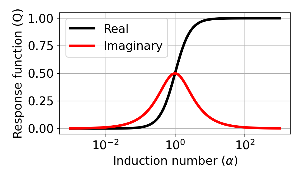
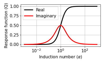
The Response Function is a complex quantity and the real and imaginary parts (or in-phase and quadrature phase) look like below figure. The horizontal axis is the induction number.
(Source code, png, hires.png, pdf)
Eq. (367) has two main components. \(C\) is determined by geometry. \(Q\) relates to the target body.
In the following pages we illustrate