Understanding the Harmonic EM response

The EM response from a buried loop

\[\begin{split}\frac{H_3^s }{H_3^p} = \frac{\mathcal{E}_3^s }{\mathcal{E}_3^p} = - \frac{M_{12}M_{23}}{M_{13}L} \Big[\frac{\alpha^2 + \imath \alpha}{1+\alpha^2}\Big] \\ = C Q (\alpha)\end{split}\]

This expression has two parts. C depends upon geometry (coupling coefficient) and Q depends only on the EM properties of the body.

• Coupling coefficient: \(C\)

• Response function: \(Q\)

Coupling coefficient

The coupling coefficient can be written as

\[C = - \frac{M_{12}M_{23}}{M_{13}L},\]

where \(M_{ij}\) stands for the mutual inductance between \(i\) and \(j\) loops. Deriving mutual inductance is an essential step to understand the coupling coefficient. The mutual inductance can be derived from the :ref :Biot-Savart law <biot_savart>, which gives us the magnetic field. Assume we are looking at two loops and the magnetic field due to the first loop is \(\mathbf{B}_1\) . We can calculate the flux \(\Phi_2\) of this magnetic field through the second loop as follows:

(368)\[\Phi_2 = \int \mathbf{B}_1 \cdot da_2 = M_{12} I_1.\]

This flux is then equal the mutual inductance times the current. We can solve for the mutual induction in a few more steps. Using Stokes’ Theorem and the vector potential of \(\mathbf{B}_1\), Equation (368) becomes a line integral:

(369)\[\Phi_2 = \int \mathbf{B}_1 \cdot da_2 = \int (\nabla \times \mathbf{A}_1) \cdot da_2 = \oint \mathbf{A}_1 \cdot dl_2,\]

where \(\mathbf{A}_1\) is derived using the Biot-Savart law:

(370)\[\mathbf{A}_1 = \frac{\mu_0 I_1}{4\pi} \oint \frac{dl_1}{\lvert \mathbf{r} - \mathbf{r'}\rvert^2}.\]

By subbing Equation (370) into (369), we get the following integral expression for the flux:

(371)\[\Phi_2 = \frac{\mu_0 I_1}{4\pi} \oint \left ( \oint \frac{dl_1}{\lvert \mathbf{r} - \mathbf{r'}\rvert^2} \right ) \cdot dl_2.\]

We can then write the mutual inductance between two loops as:

(372)\[M_{12} = \frac{\mu_0}{4\pi} \oint \oint \frac{dl_1 \cdot dl_2}{\lvert \mathbf{r} - \mathbf{r'}\rvert^2}.\]

There are a few significant things about Equation (372):

Note

• \(M_{12}\) depends purely on geometry, such as the size, shape, and relative positions of the two loops

• This expression does not change if we look at the flux in the first loop due to the second loop, meaning that \(M_{12} = M_{21}\). Therefore, following reciprocity staifies

\[M_{12} = \frac{\Phi_2}{I_1} = \frac{\Phi_1}{I_2}.\]

Effects of coupling coefficient

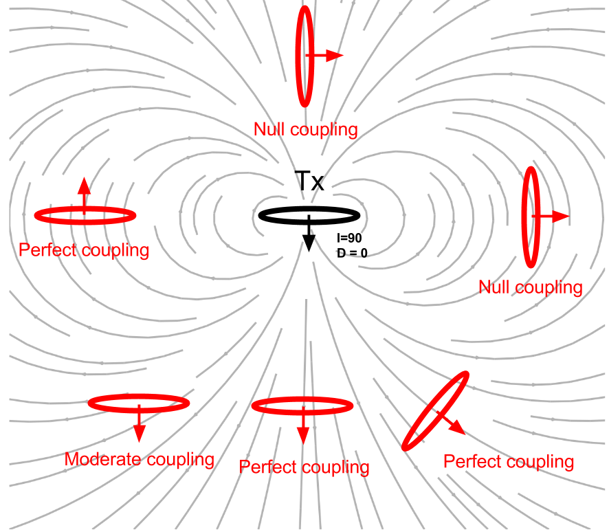
Fig. 92 Effects of coupling between loops. The orientation of the loops can be changed by adjusting the inclination I and the declination D.

Effects of the coupling coefficient (\(C\)) changes mostly due to orientation of the loops. We define orientation of a loop using inclination (\(I\)) and declination (\(D\)) as shown in Fig. 92. For detailed definitions of inclination and declination see XXX. When the orientation the Body loop is aligned with magnetic field line, better coupling is created resulting in greater mutual inductance.

We consider a set up with the three loops: Tx, Rx, and body. Left panel of Fig. 93 shows the primary field lines, and interaction between Tx and Rx, and Tx and Body. As shown in the right panel of Fig. 93, in the body, secondary magnetic field is generated, and it has the same direction to \(H^p_3\) at Rx hence the EM response (\(H^s_3 / H^p_3\)) has positive sign.

This process can be explained by mutual inductance: \(M_{13}\) will have (-) because the primary field lines mostly goes up at Rx. Similarly \(M_{12}\) and \(M_{23}\) have (+) and (-) signs, respectively. Therefore, the sign of coupling coefficient will be positive. Note that not only sign but also geometric decay is considered in the mutual inductance so as in the coupling coefficient. The coupling coefficient among three loops will change as Tx and Rx loow is moving along the surface.

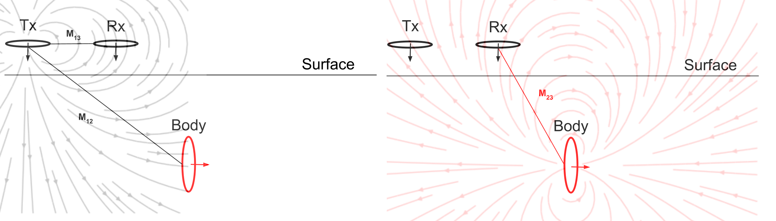
Fig. 93 Coupling between the three loops.

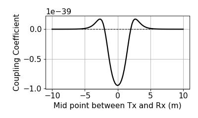
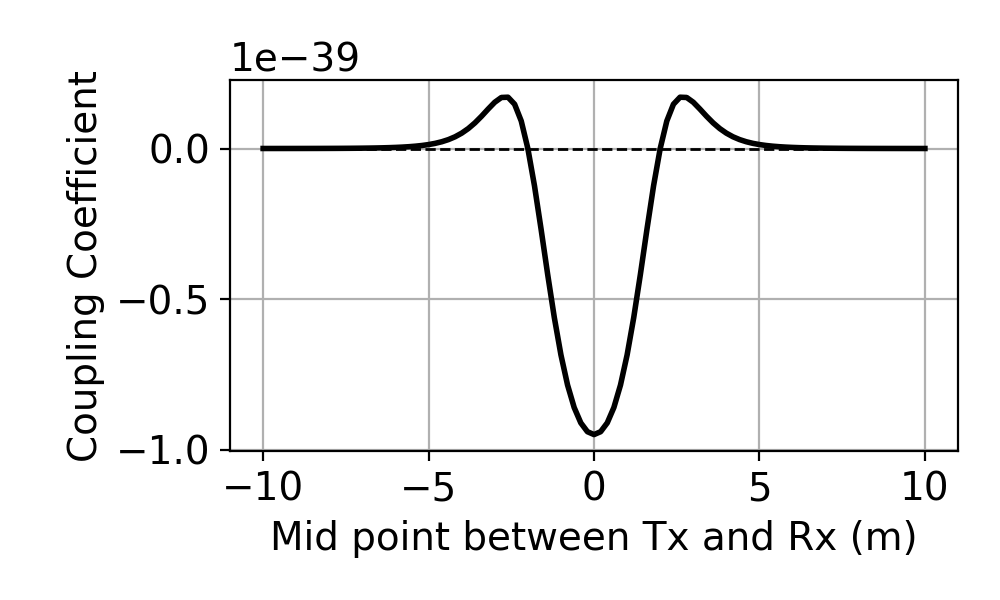
Computed coupling coefficient along the line is shown below:

(Source code, png, hires.png, pdf)

Because the coupling coefficient is generally very small, the EM response, \(\frac{H^s_3}{H^{p}_3}\) is small, regardless of the value of \(\alpha\) [0, 1]. Often part per million (ppm) is used for the unit of this ratio.

Response function

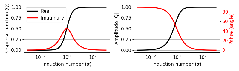
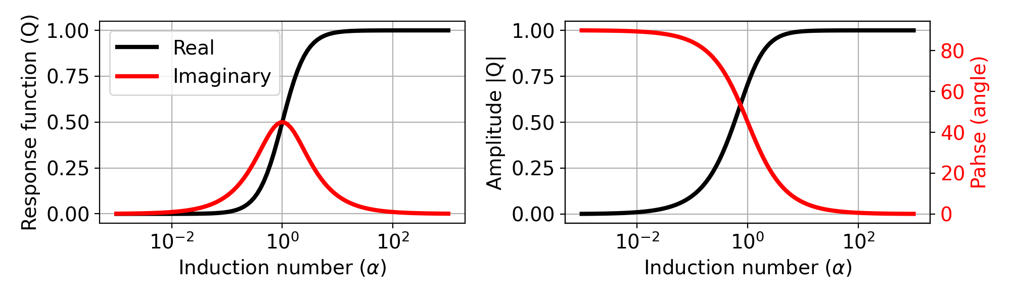
The response function, \(Q\) can be written as

\[Q = \frac{\alpha^2 + \imath \alpha}{1+\alpha^2}\]

Since \(Q\) is complex-valued, we can express them as either real and imaginary or ampliutde and phase.

(Source code, png, hires.png, pdf)

Asymptotic

We have obtained full expression of the EM response (\(H^s_3/H^p_3\)), which can be written as

\[\frac{H^s_3}{H^p_3} = - \frac{M_{12}M_{23}}{M_{13}L} \Big[\frac{\alpha^2 + \imath \alpha}{1+\alpha^2}\Big]\]

Obtaining asymptotic values of this EM response at small and large \(\alpha\) provides important physical features:

Resistive limit: when \(\alpha \ll 1\):

\[\frac{H^s_3}{H^p_3} \approx - \frac{M_{12}M_{23}}{M_{13}L} (\imath \alpha)\]

The EM response is purely imaginary-valued. The amount of current induced in the body will also be small, and the secondary magnetic field will be everywhere much smaller than the primary field. Therefore, each process of induction(Rx from Tx, body from Tx, Rx from body) can be considered as quite independently.

Note

Within the resistive limit, it is reasonable to superpose EM response from multiple bodies.

Inductive limit: \(\alpha \gg 1\):

\[\frac{H^s_3}{H^p_3} \approx - \frac{M_{12}M_{23}}{M_{13}L}\]

The EM response is purely real-valued, and only dependent of the coupling coefficient. As \(\alpha\) becomes larger, the secondary magnetic field induced an EMF in the body which begins to become appreciable in relation to that induced by the primary field. The phase angle of the current in the body, and therefore the phase angle of the secondary magnetic field, must shift in order that the net induced EMF and the resistive loss should exactly balance. At the inductive limit, this balance virtually becomes equality between the EMFs induced by the primary and by the secondary magnetic field in the body. The induced current and the secondary magnetic field must therefore be in- phase with, but in opposition to the primary field.

Phase

The phase of \(\frac{H^s_3}{H^p_3}\), \(\theta_s\) will be same as that of \(Q(\omega)\), hence

(373)\[\theta_s = - \frac{\pi}{2} - \phi,\]

where

(374)\[\phi=tan^{-1}(\frac{\omega L}{R})=tan^{-1}(\alpha).\]

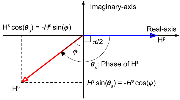
Fig. 94 Phase diagram of secondary magnetic field (\(H^s\)).

From above diagram and Eq. (374), it can be seen that:

Note

• For a very good conductor: \(\alpha = \frac{\omega L}{R} \rightarrow \infty\) and \(\phi \rightarrow \frac{\pi}{2}\). In this case, phase of the secondary field is 180 \(^\circ\) (\(\pi\)) behind the primary field

• For a very poor conductor: \(\alpha = \frac{\omega L}{R} \rightarrow 0\) and \(\phi \rightarrow 0\). In this case, phase of the secondary field is 90 \(^\circ\) (\(\frac{\pi}{2}\)) behind the primary field

Assuming the phase of the primary magnetic field, \(\theta_p=0\), its phase lag, \(\psi\), can be written as

(375)\[\psi = \theta_p - \theta_s =\frac{\pi}{2} + \phi,\]

The lag in the phase of \(\frac{\pi}{2}\) is due to the inductive coupling between Loop1 and Loop2, whereas the additional phase lag \(\phi\) is determined by the properties of the conductor as an electrical circuit. That is,

\[ \begin{align}\begin{aligned}H^s_3 = |H^s_3| cos (\omega t - (\frac{\pi}{2}+\phi)) = |H^s_3| sin (\omega t - \phi)\\ = |H^s_3| \Big( cos (\omega t-\frac{\pi}{2}) cos (\phi) + cos (\omega t-\pi) sin (\phi) \Big)\end{aligned}\end{align} \]

The component of \(H^s_3\) 180 \(^\circ\) out of phase with \(H^p\) is \(H^s_3 sin(\phi)\), whereas the component 90 \(^\circ\) out-ouf-phase is \(H^s_3 cos(\phi)\).

In frequency domain EM survey:

• the 180 \(^\circ\) out-of-phase fraction of \(H^s_3\) is called the Real or In-phase component.

• the 90 \(^\circ\) out-of-phase fraction of \(H^s_3\) is called the Imaginary, Out-of-phase, or Quadrature component.