Faraday’s Law
We can observe several characteristics of EM induction using the applet:
The voltmeter only registers a signal when the magnet is moving, regardless of its absolute position.
The sign of the induced voltage changes depending on the direction of motion and orientation of the magnet
The magnitude of the voltage depends on how quickly the magnet is moving
All else being equal, the voltage induced in the four coil loop is larger than in the two coil loop.
These behaviours are described by Faraday’s law. Faraday’s law is named after English scientist Michael Faraday (1791-1867), and describes the manner in which time-varying magnetic fields induce the rotational electric fields. This explains the electromagnetic induction phenomenon, which is a fundamental excitation mechanism of the inductive source.
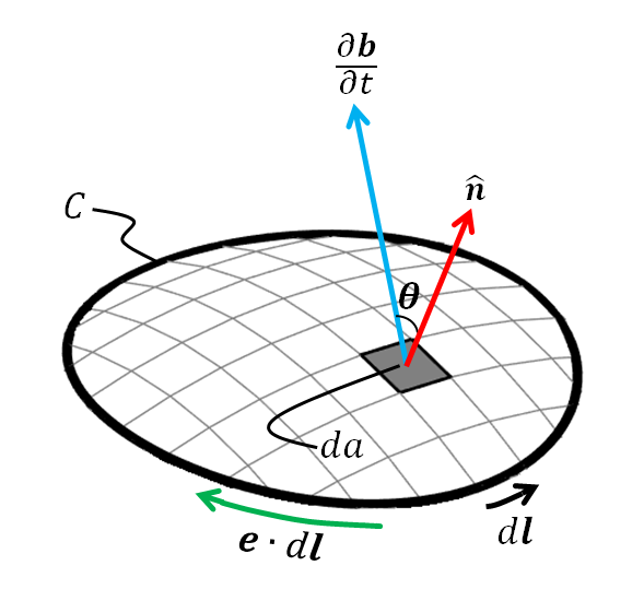
Integral Form in the Time-Domain
Faraday’s law in integral form can be expressed using the following equation:
where:
\(\mathbf{e}\) is the electric field defined around a closed path \(C\)
\(\mathbf{b}\) is the magnetic flux density defined over a closed surface \(A\) contoured by \(C\)
\(\hat n\) is an outward normal unit vector perpendicular to \(da\)
\(\ d\mathbf{l}\) is a vector element of length along contour \(C\)
Eq. (55) states that the time-dependent rate of change in magnetic flux, through a surface bounded by a closed path, is negatively proportional to the line integral of the electric field it induces over that path.
Differential Form in the Time-Domain
By applying Stokes’s theorem to left-hand side of Eq. (55), we can obtain the differential form of Faraday’s law:
Eq. (56) states that time varying magnetic fields will induce rotational electric fields. Furthermore, the curl of the induced electric fields opposes time-dependent changes in the inducing magnetic field.
Faraday’s Law in the Frequency-Domain
The frequency-domain representation of Faraday’s law can be obtained by applying a Fourier transform to Eqs. (55) and (56). The integral form of Faraday’s law in the frequency domain is:
Similarly using Stokes’ theorem, the differential form of Faraday’s law is:
where \(\omega\) is the angular frequency, \({\bf E}\) is the frequency-dependent electric field and \({\bf B}\) is the frequency- dependent magnetic flux density.
From Eq. (58) , we can infer two things:
Induced rotational electric fields are proportional to the angular frequency; this implies that electromagnetic induction is larger at higher frequencies.
Induced rotational electric fields, and the frequency-dependent magnetic fields responsible for them, are 90 degrees out of phase.
Discovery of Faraday’s Law
Faraday’s law is best understood using three experiments, which Faraday conducted and summarized in 1831. For each of these experiments, an electromagnet was used to create a time-dependent magnetic field, which we will represent using the magnetic flux density \({\bf {b}}\). A loop of wire with area \(A\), contoured by a closed path \(C\), was then held in proximity of the electromagnet. This resulted in a magnetic flux \({\boldsymbol \Phi_b}\) defined by:s
Faraday then conducted the following three experiments:
The loop of wire was mobed while the electromagnet remained stationary.
The electromagnet was moved while the loop of wire remained stationary.
Both the loop of wire and electromagnet remained stationary, however, the strength of the magnetic field was varied as a function of time.
Faraday noticed that in all three experiments, an electromotive force \(\mathcal{E}\) was induced in the wire, resulting in a measurable electric current. The electromotive force \(\mathcal{E}\) can be defined in terms of the electric field \({\bf e}\) by integrating over the path of the wire as follows:
In an ideal circuit, the electromotive force is equivalent to the Voltage \(V\) experienced by the wire. For a circuit with resistance \(R\), Ohm’s law \(V=IR\) can be used to show that electromotive forces are associated with currents \(I\). Faraday’s breakthrough came by proposing that a time-dependent change in magnetic flux through the wire loop was responsible for the resulting electromotive force. In 1833, Heinrich Lenz determined that the time dependent change in magnetic flux was negatively proportional to the electromotive force it generated. The contributions made by Faraday and Lenz are represented by the following equation:
Lenz’s contribution to Faraday’s discovery not only provides the equality in Eq. (61) , but determines the direction of force on free charges in response to changes in an applied magnetic field. For a more complete description see the Lenz’s Law page. By substituting the definition of magnetic flux from Eq. (59) and the definition of electromotive force from Eq. (60) into Eq. (61), we can obtain Faraday’s law in integral form according to Eq. (55) .
Units
Magnetic flux density |
\(\mathbf{b}\) |
\(\frac{\text{Wb}} {\text{m}^{2}}\) |
Weber per square meter |
Electric current density |
\(\mathbf{j}\) |
\(\frac{\text{A}} {\text{m}^{2}}\) |
Ampere per square meter |
Electric field intensity |
\(\mathbf{e}\) |
\(\frac{\text{V}} {\text{m}}\) |
Volt per meter |
Electric potential |
\(\text{V}\) |
V |
Volt |
Electromotive force |
\(\mathcal{E}\) |
V |
Volt |
Electric current |
\(\text{I}\) |
A |
Ampere |
Consider the units of quantities on the left and right-hand sides of Eq. (55). Using dimensional analysis, we obtain:
Therefore the above expression states that a change in magnetic flux, equal to 1 Weber per second, will induce an electromotive force of 1 Volt along a closed path. Using the aforementionned expression, the Weber (\(Wb\)) can be expressed as:
where \(J\) is the Joule, and \(A\) is Ampere. Joules are used to represent a unit of energy, or work. Thus we can interpret the magnetic flux as a unit of work per unit current.
Geophysical Applications Faraday’s Law
When performing electromagnetic surveys, various instruments are used to generate time-dependent magnetic fields. These fields are commonly refered to as primary fields. According to Eqs. (56) , this will induce rotational electric fields within the surrounding region. For a rock unit defined by conductivity \(\sigma\), Ohm’s law (\({\bf j} = \sigma {\bf e}\)) implies that a current density \({\bf j}\) is also induced by the primary field. These induced currents are parallel to \({\bf e}\) , and have a magnitude which depends on the physical properties of the rock. Therefore, we can use Faraday’s law in differential form to understand the manner in which rotational currents are induced in conductive objects, by an artificially generated primary field.
According to the Biot-Savart law Section Biot-Savart, current densities are responsible for generating magnetic fields. This implies that currents induced by the primary field will result in the creation of an anomalous magnetic field, commonly refered to as the secondary field. The secondary field can be measured at locations above the Earth’s surface, and provides important information regarding subsurface geological structures. But how is the secondary field measured?
If placed in a region where secondary fields are observable, a receiver loop of wire will experience an electromotive force according to Eq. (61) . From Eq. (60), and we know that the electromotive force is equivalent to the voltage being induced in the wire. Therefore we can use voltage measurements to represent information regarding the secondary field, as opposed to measuring the field directly.
The explanation provided in this section may also be understood in the frequency-domain. However, the voltage induced within the receiver coils will have both real (in-phase) and imaginary (out-of-phase) components.