Solving Maxwell’s Equations
Purpose
Here, we provide a general overview on how to solve Maxwell’s equations in practice. The approaches used to solve specific problems are covered later in EM GeoSci.
The practice of solving Maxwell’s equations for an applied problem can be broken into three parts:
Defining the problem: here, Maxwell’s equations are modified, reformulated or approximated to suite a particular physical problem.
Setting boundary and initial conditions: these are invoked so that solutions to Maxwell’s equations are uniquely solved for a particular application.
Solving with analytic or numerical approaches: once the problem, boundary conditions and initial conditions have been defined, the final solution is obtained through analytic or numerical approaches.
Defining the Problem
In “Overview of Maxwell’s Equations”, we presented general formulations for Maxwell’s equations. In most cases however, Maxwell’s equations can be modified, reformulated or approximated to simplify an applied problem. Failure to choose an appropriate formulation may result in the problem being difficult or impossible to solve using current means.
Examples (to be discussed in more detail throughout EM GeoSci):
where \(\mathbf{J_s}\) is an electrical current source and \(\phi\) is a scalar potential.
where \(\mathbf{J_s}\) is an electrical current source. For some problems, we may be able to work in the quasi-static (\(\sigma \gg \omega \varepsilon\)) or wave (\(\sigma \ll \omega \varepsilon\)) regimes; allowing us to neglect terms involving \(\varepsilon\). In many geological environments, the impact of the Earth’s magnetic properties is negligible (i.e. \(\mu\approx \mu_0\)). In this case, we can take \(\mu\) out of the curl-curl system. In the case of a magnetic source, we would need to solve a different system.
where \(\mathbf{j_s}\) is an electrical current source. This equation is the time-dependent equivalent to the one used in frequency domain electromagnetics. For some problems, we may be able to work in the quasi-static or wave regimes; allowing us to neglect terms involving \(\varepsilon\). If the impact of the Earth’s magnetic properties is negligible (i.e. \(\mu\approx \mu_0\)), we can take \(\mu\) out of the curl-curl system. In the case of a magnetic source, we would need to solve a different system.
Boundary and Initial Conditions
Boundary Conditions
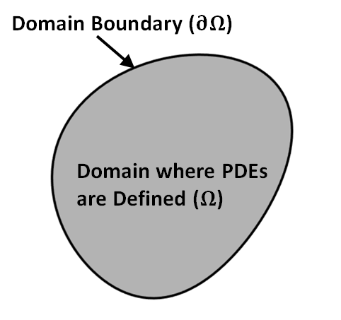
Fig. 75 Illustration of domain and boundary.
Boundary conditions ensure that a the problem is well-posed; that is, it has a unique solution. This is necessary when using Maxwell’s equations to solve applied problems in electromagnetic geosciences. Differential equations corresponding to a physical problem are defined within a region, or “domain” (denoted by \(\Omega\)). To make the problem well-posed, boundary conditions are applied to the edges of this domain (denoted by \(\partial \Omega\)). There are three types of boundary conditions, which are listed below:
Dirichlet Boundary Conditions: Dirichlet boundary conditions are by far the most straightforward and easy to implement. Dirichlet conditions directly define the value of the solution on the boundary, i.e.:
where \(\mathbf{F}\) is some vector field/flux defined within the domain, \(\mathbf{g}\) is a spatially-dependent function and \(\mathbf{r} = (x,y,z)\). In many cases, the Dirichlet condition is given as a constant value; such as, all fields go to zero at the boundary.
Neumann Boundary Conditions: Neumann boundary conditions are imposed by specifying the spatial derivatives of the solution on the boundary. Commonly, Neumann conditions define the directional derivatives normal to the surface of the domain, i.e.:
where \(\mathbf{n}\) is the unit vector direction perpendicular to the domain boundary \(\partial \Omega\), \(F_n = \mathbf{F \cdot \hat n}\;\) is the component of a vector field/flux \(\mathbf{F}\) along \(\mathbf{n}\), \(\mathbf{g}\) is a spatially-dependent function and \(\mathbf{r} = (x,y,z)\). Physically, Neumann conditions are used to define the rate of flux through the boundary. This is frequently applied to problems which behave according to the heat equation.
Robin (Mixed) Boundary Conditions: Robin boundary conditions are a linear combination of Dirichlet and Neumann conditions, i.e.:
where \(a\) and \(b\) are constants, \(\mathbf{n}\) is the unit vector direction perpendicular to the domain boundary \(\partial \Omega\), \(F_n = \mathbf{F \cdot \hat n}\;\) is the component of a vector field/flux \(\mathbf{F}\) along \(\mathbf{n}\), \(\mathbf{g}\) is a spatially-dependent function and \(\mathbf{r} = (x,y,z)\). Robin conditions are used when the rate of flux leaving the domain is dependent on the value of the field at the boundary.
Initial Conditions
Initial conditions, in addition to boundary conditions, are required to solve time-dependent problems. Because the solutions to problems in the physical sciences are causal, the fields and fluxes at a particular time depend on the fields and fluxes at earlier times. Generally, we set initial conditions to define the solution at \(t=0\) and we are interested in the bahaviour of the fields and fluxes at \(t\geq 0\). If the differential equation being solved has only first order derivatives in time, initial conditions may be given by:
where \(\mathbf{F}\) is a vector field/flux and \(\mathbf{F_0}\) is the vector field/flux at \(t=0\). This type of condition would be needed to solve the time-domain electromagnetic equation presented in “Defining the Problem”.
Multiple Variables and Higher Order Time-Derivatives
If the differential equation contains multiple variables and higher order time-derivatives, we cannot solve the problem by simply setting initial conditions on the fields/fluxes at \(t=0\). Where \(k\) is the highest order time-derivative found in the problem and \(n\) is the number of time-dependent variables, we would require \(nk\) total initial conditions to solve the problem. These initial conditions would take the form:
where \(\mathbf{F}\) is the vector field/flux associated with variable \(n\), and \(\mathbf{g^k}\) is a time-dependent function defined throughout the entire domain for the \(k^{th}\) derivative. An example of this is the time-dependent wave equation presented in “Defining the Problem”, which requires initial conditions on both \(\mathbf{e}\) and its first-order time-derivative \(\partial \mathbf{e}/\partial t\).
Analytic and Numeric Solutions
Having formulated Maxwell’s equations appropriately, as well as implementing boundary conditions and initial conditions, we can now solve the problem. There are two ways in which meaningful solutions can be obtained: analytically and numerically.
Analytic Solutions
Ideally, one would derive an analytic solution. The problem becomes even more tractable if the solution is a closed-form expression; can be evaluated using a finite number of simple operations. Analytic solutions are generally only possible if the problem is simplified or exhibits a sufficient degree of geometric symmetry. We prefer analytic solutions because they are rapid to compute and explicitly show how the solution depends on its input variables.
Some solutions may be called semi-analytic. Semi-analytic solutions generally require the numerical evaluation of one or more integral functions, infinite series and/or limits. In this case, the solution is not a closed form expression. However, semi-analytic solutions can be very useful in practice.
Numerical Solutions
Numerical solutions are used to approximate the fields and fluxes to a desired level of accuracy. Numerical approaches are able to solve problems without relying on geometric symmetries. The process of obtaining a numerical solution can be broken down into three parts:
Discretizing the Domain
Defining Fields and Fluxes
Applying Computer Algorithms
A conceptual understanding of the aforementioned steps will be provided here. However, we will not present all the required background for solving these problems in practice; as it is extensive.
Discretizing the Domain:
In order to obtain a numerical solution, the domain is first discretized; i.e. subdivided into a collection of small volumes/regions. The collection of these volumes is called a ‘mesh’. The physical properties within each volume are considered constant. The size and shape of each volume depends on the geometry of the problem, the size of the domain and the quantity of available computer memory. In Fig. 76 a, we see a 1D discretization. The 1D discretization works well when, locally, the Earth displays a layered structure. For problems with irregular geometries, we may choose to use a 2D or 3D discretization (Fig. 76 b). As a rule, the finer the discretization (as the dimensions of the cells decrease), the better our numerical solution will approximate the true solution to our problem.
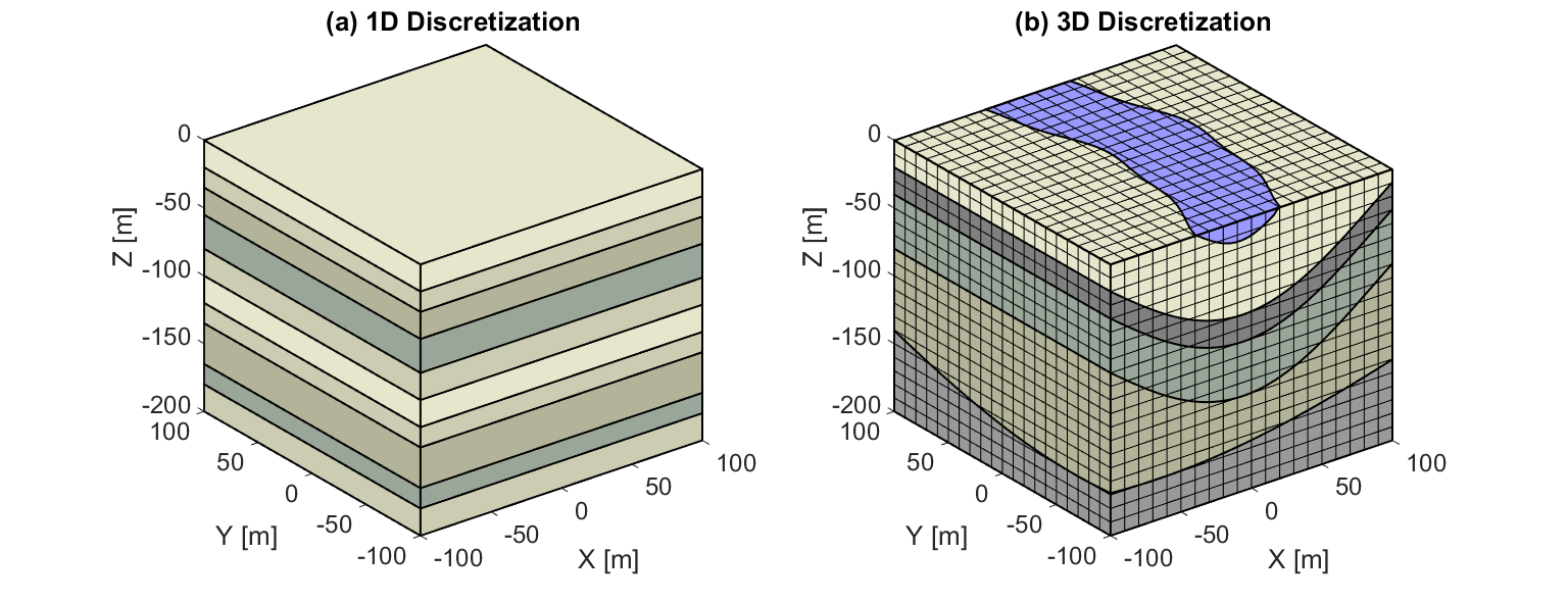
Fig. 76 Discretization of Earth’s structure. (a) 1D discretization. (b) 3D discretization.
Defining Fields, Fluxes and Potentials
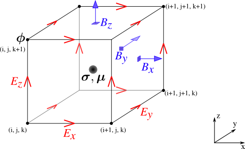
Fig. 77 Definition of fields (\(\mathbf{E}\)), fluxes (\(\mathbf{B}\)) and potentials \(\phi\) on a cubic cell.
The fields, fluxes and/or potentials pertaining to a particular problem are defined throughout the entire domain. Once the domain has been discretized however, evaluation of these quantities is only possible at a finite number of locations. The fields, fluxes and/or potentials being computed depend on the formulation of Maxwell’s equations. The locations of these quantities for each cell depend both on the problem and the corresponding interface conditions.
As an example, consider Fig. 77 where:
the potential \(\phi\) is defined on the cell nodes.
cartesian components of the electric field \(\mathbf{E}\) are defined on the cell edges.
cartesian components of the magnetic flux density \(\mathbf{B}\) are defined on the cell faces.
physical properties \(\sigma\) and \(\mu\) are defined at the cell centers.
For problems involving \(\mathbf{E}\) and \(\mathbf{B}\), this approach is ideal because it naturally respects the interface conditions for electromagnetic fields. Recall from “Interface Conditions” that tangential components of the electric field and normal components of the magnetic flux are continuous are continuous across interfaces.
Applying Computer Algorithms:
As a final step, the numerical problem is commonly written as a linear system and solved using computer algorithms. The system can be formed using finite difference, finite volume or finite element methods. It generally takes the form:
where \(\mathbf{u}\) contains the fields and/or fluxes at discrete locations throughout the domain, \(\mathbf{q_s}\) is a vector corresponding to the source term and \(\mathbf{A(m)}\) is a linear operator that depends on the physical properties (\(\sigma,\mu,\varepsilon\)). Collectively, the physical properties defining each cell make up a physical property model \(\mathbf{m}\). In electromagnetic geosciences, we are frequently interested in the “inverse problem”. That is, can we recover the physical property model \(\mathbf{m}\) if \(\mathbf{u}\) and \(\mathbf{q_s}\) are known?