General Formulation

Purpose

Here, we present analytic expressions according to Wait and Spies ([WS69]). These expressions can be used to predict the time-dependent dipole response from a conductive and magnetically permeable sphere in free-space.

Problem Geometry

Fig. 137 Problem geometry for a conductive and magnetically permeable sphere in free-space.

Fig. 138 Dipolar response \(\mathbf{h} (t)\) (purple) from a conductive and magnetically permeable sphere, under the influence of a spatially uniform field \(h_0 (t)\) (red). The induced dipole moment (blue) is represented by \(\mathbf{m} (t)\).

Consider the illustration in Fig. 137. Here, a sphere of radius \(R\), conductivity \(\sigma\) and magnetic permeability \(\mu\) is located in the vicinity of an inductive source transmitter (\(Tx\)). The transmitter generates a time-dependent primary field \(\mathbf{h_0} (t)\) which induces an excitation within the sphere. The excitation induced within the sphere produces a secondary field \(\mathbf{h_s} (t)\) which is then measured by a receiver coil (\(Rx\)). Note that because we are in free-space, \(\mathbf{h_0} (t)\) may be calculated using the Biot-Savart law.

To approximate the sphere’s response, Wait and Spies ([WS69]) considered the dipole response from a conductive and magnetically permeable sphere under the influence of a spatially uniform field. The geometry of this problem is illustrated in Fig. 137. The transmitter’s primary field may be considered spatially uniform about the sphere if 1) the radius of the sphere is much smaller than the wavelength of the inducing field, and 2) the distance between the transmitter and the sphere is sufficiently larger than the sphere’s radius (typically \(> 10R\)). According to Wait and Spies ([WS69]), the sphere’s free-space dipole response \({\bf h} (t)\) can be expressed in terms of a time-dependent dipole moment \({\bf m}(t)\) such that:

(432)\[{\bf h} (t) = \frac{1}{4\pi} \Bigg [\frac{3{\bf r} [ \, {\bf m}(t) \cdot {\bf r}\, ]}{r^5} - \frac{{\bf m}(t)}{r^3} \Bigg ]\]

where \({\bf r}\) is the vector distance between \({\bf P}\) and \({\bf Q}\). The induced magnetic dipole moment for the sphere’s excitation is given by the following convolution:

(433)\[{\bf m}(t) = \frac{4\pi}{3}R^3 \chi (t) \otimes {\bf h_0} (t)\]

where \(\chi (t)\) represents an impulse response for the sphere’s induced dipole moment. The impulse response is defined as the inverse Fourier transform of the sphere’s frequency-dependent excitation factor \(\chi (i \omega)\). An explicit expression for \(\chi (t)\) can be obtained from Wait and Spies ([WS69]):

(434)\[\chi (t) = - \frac{3}{2} \delta (t) + \frac{3}{2} \Bigg ( \frac{6 \mu_r}{\beta^2} \sum_{n=1}^\infty \frac{\xi_n^2 e^{-\xi_n^2 \, t/\beta^2}}{(\mu_r + 2)(\mu_r - 1) + \xi_n^2} \Bigg ) u(t)\]

where \(u(t)\) is the unit-step function, \(\delta (t)\) is the Dirac delta function, \(\mu_r = \mu/\mu_0\) is the relative permeability of the sphere and:

(435)\[\beta = \big ( \mu \sigma \big )^{1/2} R\]

Coefficients \(\xi_n\) within the sum are defined by:

(436)\[\textrm{tan} \, \xi_n = \frac{(\mu_r - 1)\xi_n}{\mu_r - 1 + \xi_n^2}\]

These coefficients are spaced roughly \(\pi\) apart with:

(437)\[n\pi \leq \xi_n \leq (n+1/2) \pi\]

In practice, the value of each coefficient may be found iteratively using very few iterations (< 10) according to:

(438)\[\xi_n^{(k+1)} = n\pi + \textrm{tan}^{-1}\Bigg ( \frac{(\mu_r - 1) \xi_n^{(k)}}{\mu_r - 1 + (\xi_n^{(k)} )^2} \Bigg )\]

Therefore, we can predict the sphere’s dipole response by performing the following operations. First, the impulse response defined in Eq. (434) is determined for a particular sphere. Although it is expressed as an infinite sum, only a finite number of terms are needed; as the contribution of each term decays with respect to \(n\). The \(\xi_n\) coefficients used to approximate the sum are determined individually using Eq. (438), with an initial value according to (437). For a particular inducing field \(h_0(t)\), the convolution in Eq. (433) is evaluated numerically for a set of times. After a numerical approximation for the magnetic dipole moment is obtained, the time-dependent response at a particular location is predicted according to Eq. (432).

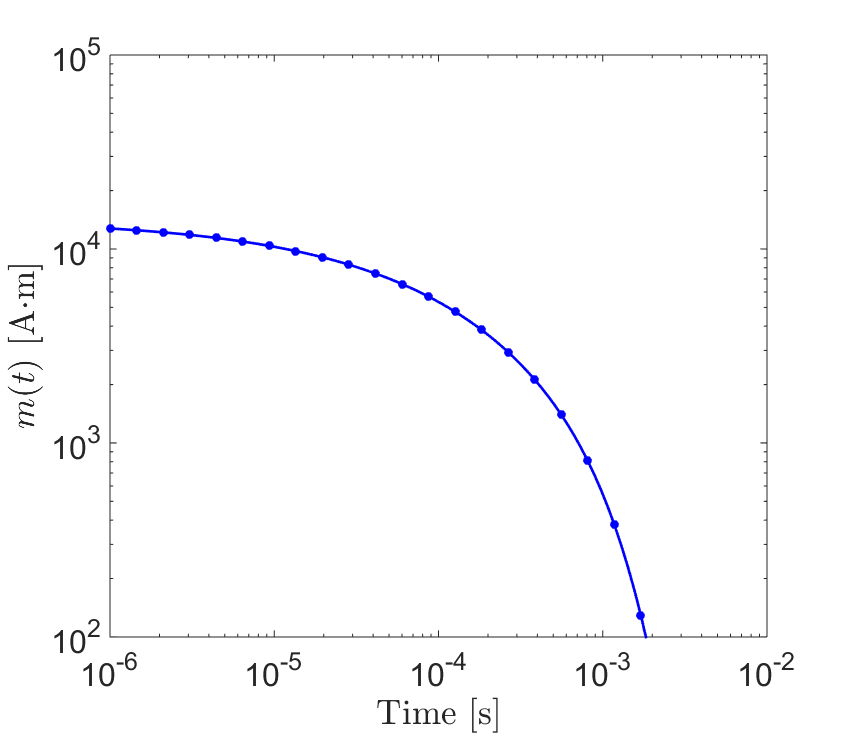
Fig. 139 Transient dipole moment at \(t>0\) for a sphere of radius \(R\) = 10 m, conductivity \(\sigma\) = 10 S/m and relative permeability \(\mu_r\) = 6.

As an example, let us consider a sphere of radius \(R=10\) m, conductivity \(\sigma = 10\) S/m and relative permeability \(\mu_r=6\). The sphere has been subjected to a static inducing field with magnitude \(h_0=1\) A/m since \(t = -\infty\). At \(t=0\) s, the field is removed; which induces a time-dependent excitation within the sphere. This particular excitation defines the sphere’s transient or “step-off” response. The magnetic dipole moment which characterizes the sphere at \(t>0\) is shown in Fig. 139.

The sphere’s step-off response depends on the dimensions and physical properties of the sphere. These dependencies are discussed in the following section for permeable and non-permeable spheres.