Circuit Model for EM Induction
Purpose
We expand EM response derived from the circuit model in frequency domain to time domain.
The basic EM survey is shown in Fig. 134. The time varying magnetic field (referred to as the primary field) in the Tx induces currents in the conductor. Those currents produce a secondary field that can be recorded at the receiver.
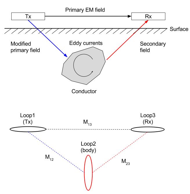
Fig. 134 Conceptual diagrams for EM inductions. Top panel shows excitation of the conductor using induction, and botton panel shows corresponding 3-loops system.
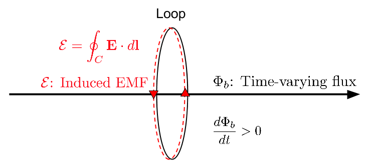
From Faraday’s Law, we establish the link between EMF (\(\mathcal{E}\), voltage), and time varying flux (\(\Phi_b\)). Below diagram illustrates how EMF could be generated from time-varying flux (\(\mathcal{E}= - \frac{d \Phi_b}{dt} = \imath \omega \Phi_b\)). The EMF (voltage) produces a current in the loop.
The circuit model is now understood as follows:
Loop 1: is the transmitter (Tx). It has a time varying current (often a step-off current in time domain: \(I_1 (1-u(t))\)) and hence produces a time varying field everywhere in space. Here \(u(t)\) indicates Heaviside step function. This is the main difference in time domain response compared to frequency domain using sinusoidal current.
Loop 2: represents the conductive body. The time varying flux generates currents in the conductor (\(I_2 (t)\)). These time varying currents produce a time varying field everywhere in space.
Loop 3: is the receiver (Rx). The measured EMF, \(\mathcal{E}^t\) is
\[\mathcal{E}^t = \mathcal{E}^p +\mathcal{E}^s\]where superscripts refer respectively to the total, primary, and secondary fields.
In time domain, primary and secondary voltage at the Loop due to step-off current can be expressed as
Here, \(M_{ij}\) is the mutual inductance between loops \(i\) and \(j\), \(L\) is the self inductance of the target loop.
Note
The terms in these equations do not separate quite as neatly as in the frequency domain (\(\mathcal{E}^s / \mathcal{E}^p = CQ\)). All have dimensions, so scale is important in time domain.
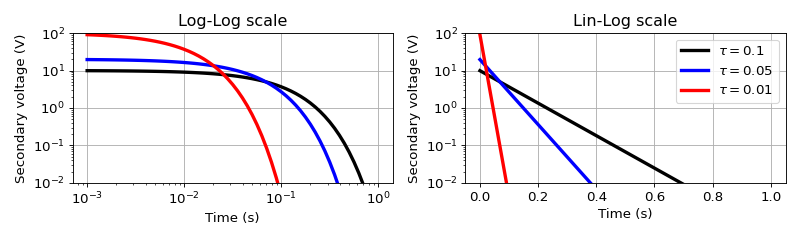
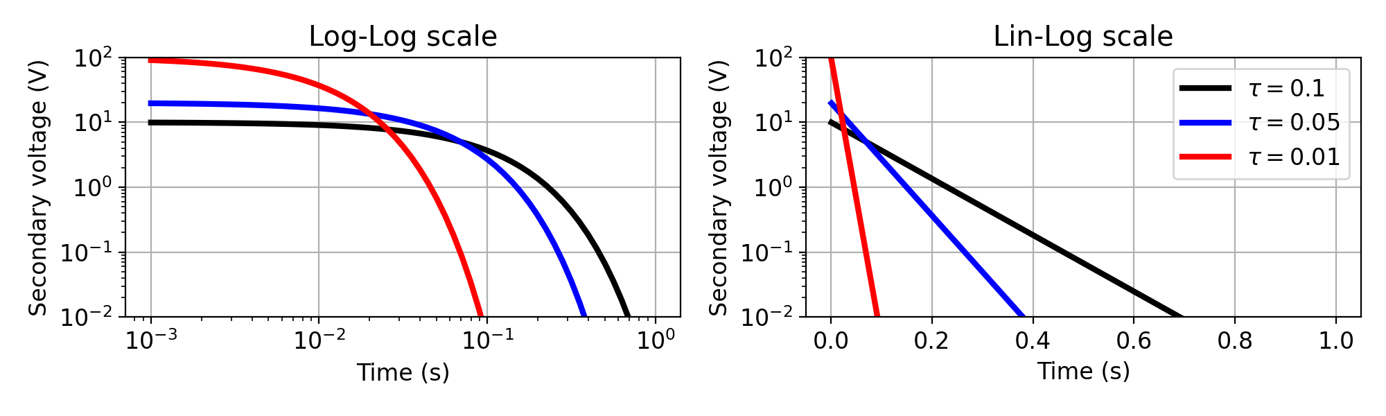
Below shows secondary voltage with variable \(\tau\) in Log-Log and Lin- Log plot. In the Lin-Log plot, exponential decay will be straight line.
(Source code, png, hires.png, pdf)

In the following pages we illustrate