Transient responses

Purpose

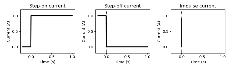
Understand relationship between transient (TDEM) and harmonic (FDEM) responses. Differentiate standard types of transient responses: a) step-on, b) impulse, and c) step-off.

(Source code, png, hires.png, pdf)

Step-on response

Often time domain EM method utilize a transient primary field rather than an alternating (or sinusoidal) one. That is, the source varies stepwise in time (TDEM) than varies harmonically (FDEM). We consider the theoretical connections between two types of response.

A unit-step function (same as Heaviside step function) can be written in a spectral form:

\[u(t) = \frac{1}{2 \pi} \int_{-\infty}^{\infty} U (\omega) e^{\imath \omega t}d \omega\]

where \(\omega\) is angular frequency (rad/s) and \(U(\omega)\) is the spectrum of \(u(t)\) and is given by

\[\begin{split}U(\omega) = \int_{-\infty}^{\infty} u(t) e^{-\imath \omega t} d t \\ = \int_{0}^{\infty} u(t) e^{-\imath \omega t} d t\end{split}\]

Although the latter integral is divergent, it can be evaluated by introducing a damping facttor \(e^{-pt} \ (p>0)\) and taking limit:

\[U(\omega) = \lim_{p \rightarrow 0} \int_{0}^{\infty} u(t) e^{-\imath \omega t} e^{-pt} d t = \frac{1}{\imath \omega}\]

If the Fourier transform of \(u(t)\) is \(\frac{1}{\imath \omega}\) then it is clear that the transformation of the secondary field \(h^s_{on}\) produced by a step-on current: \(I u(t)\) is related to the response \(H^s (\omega) e^{\imath \omega t}\) due to a sinusoidal current: \(I e^{\imath \omega t}\) as follows:

(431)\[h^s_{on}(t) = \frac{1}{2 \pi} \int_{-\infty}^{\infty} \frac{H^s(\omega)}{\imath \omega} e^{\imath \omega t} d \omega\]

From (431), computing transient response, \(h^s_{on}\) is possible with full spectrum of harmonic response, \(H^s(\omega)\). Conversely, we know from the Fourier theorem:

\[\frac{1}{\imath \omega} H^s(\omega) = \int_{-\infty}^{\infty} h^s_{on}(t) u(t) e^{-\imath \omega t} d t\]

and thus

\[H^s(\omega) = \imath \omega \int_{0}^{\infty} h^s_{on}(t) e^{-\imath \omega t} d t\]

Therefore, the harmonic response is computable if the transient response \(h^s_{on}(t)\) is known for \(t>0\).

Impulse response

Impulse response indicates that we put Dirac-Delta function as a current, which corresponds steady-state source in frequency domain (\(Ie^{\imath \omega t}\)). Note that Fourier transform of \(Ie^{\imath \omega t}\) is \(I\delta(t)\), where \(\delta(t)\) is Dirac-Delta function.

From step-on response \(h^s_{on}(t)\), we can simply obtain impulse response \(h^s(t)\)

\[h^s(t) = \frac{\partial h^s_{on}(t)}{\partial t}\]

or it can be defined with Fourier transform

\[h^s(t) = \frac{1}{2 \pi} \int_{-\infty}^{\infty} H^s(\omega) e^{\imath \omega t} d \omega\]

Conversely, from the impulse response, step-on response can be defined as

\[h^s_{on}(t) = \int_{0}^t h^s(\tau) d \tau\]

Step-off response

For practical applications, common current waveform is closer to step-off rather than step-on. Step-off waveform can be defined as

\[u(-t) = 1-u(t)\]

Then step-off response \(h^s_{off}(t)\) can be

\[\begin{split}h^s_{off}(t) = \int_{0}^{\infty} h^s(\tau) d \tau - \int_{0}^t h^s(\tau) d \tau \\ = h^s_{on}(\infty) - h^s_{on}(t), \ \ t > 0\end{split}\]

Thus the derivative of \(h^s_{off}(t)\) with respect to time is \(-h^s(t)\), which is the negative of the impulse response. In the following section, we discuss transient responses from the circuit model.