Derivation

General Solution for a Planewave

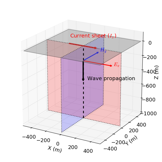
Fig. 52 Geometry of an EM plane wave propagating downwards.

To obtain a solution for EM planewaves within a homogeneous medium, let us begin with the following vector wave equations for \(\mathbf{e}\) and \(\mathbf{h}\):

(123)\[\begin{split}\boldsymbol{\nabla}^2 \mathbf{e} - \mu\epsilon \frac{\partial^2 \mathbf{e}}{\partial t^2} - \mu\sigma \frac{\partial \mathbf{e}}{\partial t} &= 0\\ \boldsymbol{\nabla}^2 \mathbf{h} - \mu\epsilon \frac{\partial^2 \mathbf{h}}{\partial t^2} - \mu\sigma \frac{\partial \mathbf{h}}{\partial t} &= 0\end{split}\]

For simplicity, let us assume that the planewave propagates along the z-direction. According to Griffiths [Gri99] (pp. 378), the electric and magnetic fields supported by a planewave are transverse to the direction of propagation; thus the electric and magnetic fields lie in the xy-plane. In this case, the governing equation for the electric field simplifies to:

\[\frac{\partial^2 \mathbf{e}}{\partial z^2} - \mu\epsilon \frac{\partial^2 \mathbf{e}}{\partial t^2} - \mu\sigma \frac{\partial \mathbf{e}}{\partial t} = 0\]

where \(\mathbf{e} \equiv \mathbf{e}(z,t)\); thus it does not depend on x or y. In order to provide initial conditions for the PDE, let the electric field be caused an impulse such that our initial conditions are given by:

(124)\[\mathbf{e}(t=0)=\mathbf{E}_0\delta(t)\]

where \(\delta(t)\) is a Dirac-Delta function at \(t=0\). Instead of solving the time-depend PDE directly, we will apply the inverse Laplace transform to analytic solutions derived in the frequency-domain:

(125)\[\mathbf{E} = \mathbf{E}_0^- e^{ikz} + \mathbf{E}_0^+ e^{-ikz}\]

where \(E_0^-\) and \(E_0^+\) are the vector amplitudes of down-going and up-going waves, respectively. Note that the harmonic term \(e^{-i\omega t}\) term is being supressed. The time domain solution for an impulse excitation can be expressed as:

\[\mathbf{e}(t) = \mathcal{F}^{-1}[\mathbf{E}(\omega)]\]

where \(\mathcal{F}[\cdot]\) is the Fourier transform. Modified from [WH88], the corresponding time domain solution for the wave equation is:

(126)\[\begin{split}\mathbf{e}(t) =& \mathbf{E}_0^- \Bigg ( e^{a(z/c)} \delta \bigg ( t+\frac{z}{c} \bigg ) -\frac{aze^{-at}}{c \big ( t^2-\frac{z^2}{c^2} \big)^{1/2}} I_1 \Bigg [ a \bigg ( t^2-\frac{z^2}{c^2} \bigg )^{1/2} \Bigg ] u \bigg ( t+\frac{z}{c} \bigg ) \Bigg ) \\ &+ \mathbf{E}_0^+ \Bigg ( e^{-a(z/c)} \delta \bigg ( t-\frac{z}{c} \bigg ) +\frac{aze^{-at}}{c \big ( t^2-\frac{z^2}{c^2} \big)^{1/2}} I_1 \Bigg [ a \bigg ( t^2-\frac{z^2}{c^2} \bigg )^{1/2} \Bigg ] u \bigg ( t-\frac{z}{c} \bigg ) \Bigg )\end{split}\]

where

• \(u(t)\) is the heaviside step function

• \(I_1(x)\) is the modified Bessel function of the first kind

• \(a=\dfrac{\sigma}{2\epsilon}\)

• \(c=\dfrac{1}{\sqrt{\mu\epsilon}}\)

Both the up-going and down-going waves have two terms. The first term, containing the Dirac delta function, is the wave term. The second term is the diffusion term. Constants \(a\) and \(c\) control both the wave and diffusion properties of the plane wave.

In the case that the EM wave were caused by an impulse corresponding to initial conditions \(\mathbf{h}(t=0) = \mathbf{H_0}\delta (t)\), the general solution for the magnetic field would be given by:

(127)\[\begin{split}\mathbf{h}(t) =& \mathbf{H}_0^- \Bigg ( e^{a(z/c)} \delta \bigg ( t+\frac{z}{c} \bigg ) -\frac{aze^{-at}}{c \big ( t^2-\frac{z^2}{c^2} \big)^{1/2}} I_1 \Bigg [ a \bigg ( t^2-\frac{z^2}{c^2} \bigg )^{1/2} \Bigg ] u \bigg ( t+\frac{z}{c} \bigg ) \Bigg )\\ &+ \mathbf{H}_0^+ \Bigg ( e^{-a(z/c)} \delta \bigg ( t-\frac{z}{c} \bigg ) +\frac{aze^{-at}}{c \big ( t^2-\frac{z^2}{c^2} \big)^{1/2}} I_1 \Bigg [ a \bigg ( t^2-\frac{z^2}{c^2} \bigg )^{1/2} \Bigg ] u \bigg ( t-\frac{z}{c} \bigg ) \Bigg )\end{split}\]

Note that Eq. (126) and Eq. (127) have the exact same form.

Note

Eqs. (126) and (127) are still general solutions, as only initial conditions have been applied. To determine \(\mathbf{E}_0^-\) and \(\mathbf{E}_0^+\) or \(\mathbf{H}_0^-\) and \(\mathbf{H}_0^+\), you must envoke a set of boundary conditions. For example, \(\mathbf{e}(z \rightarrow -\infty,t) = 0\) in addition to \(\mathbf{e}(t=0) = \mathbf{E}_0 \delta (t)\) results in a downward propagating electric field.

Supporting Derivation for the App

Fig. 53 Setup diagram of plane EM wave propagation heading downward (negaitve \(z\)).

The app simulates the downward propagation of an EM planewave due to an impulse current. As we can see in Fig. 53, the planewave is polarized such that the electric lies along the x-direction and the magnetic field lies along the y-direction. Physically, we can think of this wave as being caused by a horizontal impulse current \(\mathbf{I}(t) = I_0 \delta (t) \mathbf{u_x}\), where \(\mathbf{u_x}\) is the unit vector in the x-direction.

For the app, we only consider the quasi-static approximation of Eq. (126). This can be obtained by taking the inverse Laplace transform of the corresponding harmonic solution such that \(k = \sqrt{-i\omega\mu\sigma}\), i.e:

(128)\[\mathbf{E} (z,\omega) = E_x (z,\omega) \, \mathbf{u_x} = E_{x,0}^{-} e^{i\sqrt{-i\omega\mu\sigma}z} \mathbf{u_x}\]

where \(E_x\) is a scalar function and \(E_{x,0}^{-}\) is the scalar amplitude of the electric field. If we replace \(s=i\omega\), the inverse Laplace transform of \(E_x (z,w)\) becomes:

(129)\[\mathcal{L}^{-1}[E_x (z,\omega)] = \mathcal{L}^{-1} \Bigg [ E_{x,0}^- \, e^{- \sqrt{\mu\sigma s} z} \Bigg ]\]

If we use the following identity (Abramowitz and Stegun, 1964):

\[\mathcal{L}^{-1} \Bigg [ e^{-\alpha \sqrt{s}} \Bigg ] = \frac{\alpha}{2 \pi^{1/2} t^{3/2}} e^{-\alpha^2/4t} \;\;\; \textrm{for} \;\;\; \alpha \geq 0\]

the quasi-static solution for the electric field at \(t>0\) is given by:

(130)\[\mathbf{e}(t) = e_x(t) \mathbf{u_x} = E_{x,0}^- \frac{\big (\mu\sigma)^{1/2} z}{2\pi^{1/2} t^{3/2}} \, e^{-\mu\sigma z^2/4t} \, \mathbf{u_x}\]

Similarly, the solution for the magnetic field can be obtained by taking inverse Laplace transform of the corresponding harmonic solution such that \(k = \sqrt{-i\omega\mu\sigma}\).

\[\mathcal{L}^{-1}[H_y (z,\omega)] = \mathcal{L}^{-1} \Bigg [ - \frac{ik}{i\omega \mu} E_{x,0}^- \, e^{ikz} \Bigg ] = \mathcal{L}^{-1} \Bigg [ - \sqrt{ \dfrac{\sigma}{\mu s}} E_{x,0}^- \, e^{- \sqrt{\mu\sigma s} z} \Bigg ]\]

where \(k = \sqrt{-i\omega\mu\sigma}\), we replace \(s = i\omega\) and we let \(\sqrt{-1} = -i\). If we use the following identity (Abramowitz and Stegun, 1964):

\[\mathcal{L}^{-1} \Bigg [ \frac{1}{\sqrt{s}} e^{-\alpha \sqrt{s}} \Bigg ] = \frac{1}{\sqrt{\pi t}} e^{-\alpha^2/4t} \;\;\; \textrm{for} \;\;\; \alpha \geq 0\]

the quasi-static solution for the magnetic field is given by:

\[\mathbf{h}(t) = h_y(t) \mathbf{u_y} = -E_{x,0}^- \sqrt{\dfrac{\sigma}{\pi\mu t}}\, e^{-\mu\sigma z^2/4t} \, \mathbf{u_y}\]

where \(\mathbf{u_y}\) is the unit vector in the y-direction.