Derivation

General Solution for a Planewave

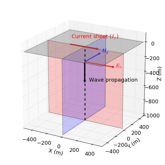
Fig. 43 Geometry of an EM planewave propagating downwards.

To obtain a solution for EM planewaves within a homogeneous medium, let us begin with the following vector Helmholtz equations for \(\mathbf{E}\) and \(\mathbf{H}\):

(112)\[\begin{split}\boldsymbol{\nabla}^2 \mathbf{E} + k^2 \mathbf{E} &= 0\\ \boldsymbol{\nabla}^2 \mathbf{H} + k^2 \mathbf{H} &= 0\end{split}\]

where the complex wavenumber is given by:

(113)\[k = \sqrt{\mu \epsilon \omega^2 - i \mu \sigma \omega}\]

For simplicity, let us assume that the planewave propagates along the z-direction. According to Griffiths [Gri99] (pp. 378), the electric and magnetic fields supported by a planewave are transverse to the direction of propagation; thus the electric and magnetic fields lie in the xy-plane. In this case, the governing equation for the electric field simplifies to:

(114)\[\frac{\partial^2 \mathbf{E}}{\partial z^2} + k^2 \mathbf{E} = 0\]

where \(\mathbf{E} \equiv \mathbf{E}(z,\omega)\); thus it does not depend on \(x\) or \(y\). The previous equation has a general solution of the form:

(115)\[\mathbf{E} = \mathbf{E}_0^- \, e^{i(kz-\omega t)} + \mathbf{E}_0^+ \, e^{-i(kz + \omega t)}\]

where \(\mathbf{E}_0^-\) and \(\mathbf{E}_0^+\) are the vector amplitudes of down-going and up-going waves, respectively. The \(e^{-i\omega t}\) in both terms controls the temporal phase. The complex wavenumber has both real and imaginary components. Thus it can be expressed as:

(116)\[k = \alpha - i\beta\]

where \(\alpha \geq 0\) and \(\beta \geq 0\) depend on the frequency and physical properties of the media. Substituting Eq. (116) into Eq. (115), the solution to our wave equation for \(\mathbf{E}\) becomes:

(117)\[\mathbf{E} = \mathbf{E}_0^- \, e^{\beta z} e^{i(\alpha z -\omega t)} + \mathbf{E}_0^+ \, e^{-\beta z} e^{-i (\alpha z + \omega t)}\]

For both the down-going and up-going waves, there are two important behaviours within the solution. The first term, which contains \(e^{\pm i \alpha z}\), controls the oscillatory behaviour (i.e. wavelength) and velocity of each wave. The second term, which contains \(e^{\pm \beta z}\), controls the decay behaviour (i.e. attenuation) of each wave. Notice that as \(z \rightarrow -\infty\) for the down-going wave, its amplitude goes to zero. The same behaviour occurs for the up-going wave as \(z \rightarrow \infty\).

Using the same approach on the Helmholtz equation for \(\mathbf{H}\), the magnetic field has a general solution of the form:

(118)\[\begin{split}\mathbf{H} &= \mathbf{H}_0^- \, e^{i(kz-\omega t)} + \mathbf{H}_0^+ \, e^{-i(kz+\omega t)}\\ &= \mathbf{H}_0^- \, e^{\beta z} e^{i(\alpha z-\omega t)} + \mathbf{H}_0^+ \, e^{-\beta z} e^{-i (\alpha z+\omega t)}\end{split}\]

Note

Eq. (117) is still a general solution. To determine \(\mathbf{E}_0^-\) and \(\mathbf{E}_0^+\) explicitly, you must envoke a set of boundary conditions. For example, \(\mathbf{E}(z \rightarrow -\infty,\omega) = 0\) and \(\mathbf{E}(z =0,\omega) = \mathbf{E}_0\). This would give you a solution \(\mathbf{E}(z,\omega) = \mathbf{E}_0 \, e^{\beta z} e^{ i(\alpha z-\omega t)}\) (i.e. just the down-going wave). From this solution, \(\mathbf{H}(z,\omega)\) can be determined using Faraday’s law. You could also envoke boundary conditions to solve for \(\mathbf{H}\) and use the Ampere-Maxwell law to obtain \(\mathbf{E}\).

Supporting Derivation for the App

Fig. 44 Downward propagating planewave modeled by the app.

The app simulates the downward propagation of an EM planewave. As we can see in Fig. 44, the planewave is polarized such that the electric lies along the x-direction and the magnetic field lies along the y-direction. Physically, we can think of this wave as being caused by a horizontal sheet of harmonic current \(\mathbf{I}(\omega) = I_x \, \textrm{cos} (\omega t) \mathbf{u_x}\), where \(\mathbf{u_x}\) is the unit vector in the x-direction.

To solve for the electric field, we begin with the general solution from Eq. (117):

\[\mathbf{E} (z,\omega) = \mathbf{E}_0^- e^{ikz} + \mathbf{E}_0^+ e^{-ikz}\]

where \(\mathbf{E}_0^-\) and \(\mathbf{E}_0^+\) are the amplitudes of the down-going and up-going waves, respectively. Given that we are only modeling the downgoing wave and the corresponding electric field only has components in the x-direction, our solution takes the form:

\[\mathbf{E} (z,\omega) = E_x (z,\omega) \, \mathbf{u_x} = E_{x,0}^{-} e^{ikz} \mathbf{u_x}\]

where \(E_x\) is a scalar function and \(E_{x,0}^{-}\) is the scalar amplitude of the electric field. Using Faraday’s law, we can confirm that the corresponding magnetic field only has components in the y-direction, where:

\[\frac{\partial E_x}{\partial z} + i \omega \mu H_y = 0\]

Solving for the y-component of the magnetic field, we obtain:

\[H_y (z,\omega ) = H_{y,0}^- e^{ikz} = -\frac{k}{\omega \mu} E_{x,0}^- \, e^{ikz}\]

Thus:

\[\mathbf{H}(z,\omega) = H_y (z,\omega) \, \mathbf{u_y} = - \frac{k}{\omega \mu} E_{x,0}^- \, e^{ikz} \, \mathbf{u_y}\]

where \(\mathbf{u_y}\) is the unit vector in the y-direction.