Transient Electric Dipole

Purpose

Here, we provide a physical description of the time-dependent electrical current dipole. This is used to develop a mathematical expression which can be used to replace the electrical source term in Maxwell’s equations. We then consider a transient electrical current dipole; which represents a more commonly used geophysical source.

General Definition

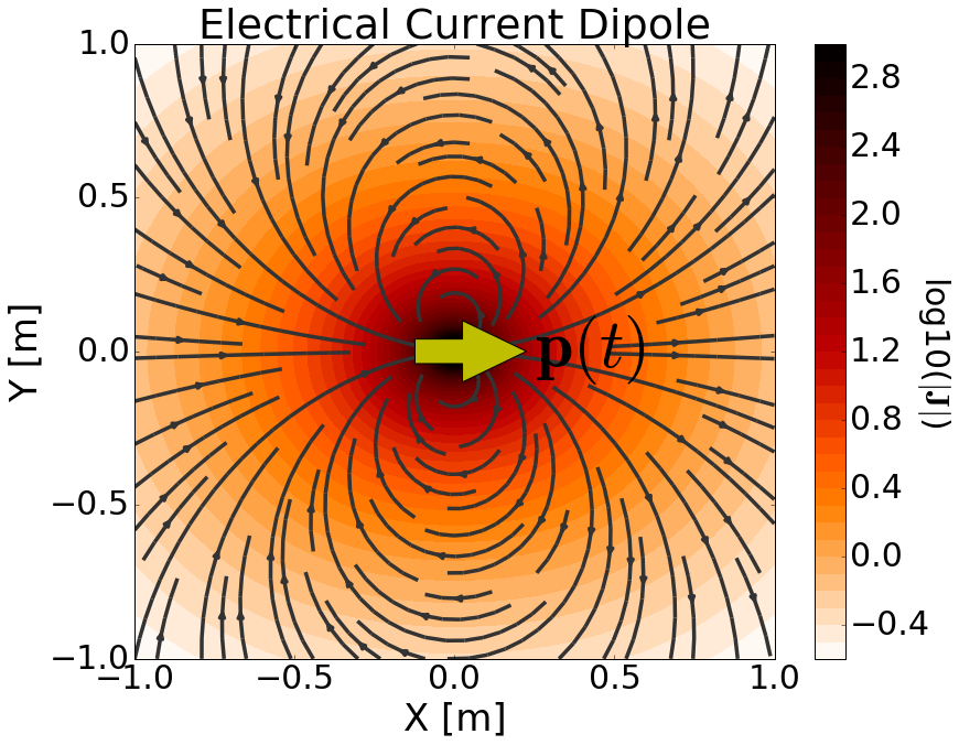
../../../../_images/E_source_current_dipole2.png — Fig. 69 Physical representation of the time-dependent electrical current dipole source.

The time-dependent electrical current dipole can be thought of as an infinitesimally short length of wire which carries a time-dependent current. The strength of the source is therefore defined by a time-dependent dipole moment \(\mathbf{p}(t)\). For a time-dependent current dipole defined by length \(ds\) and current vector \(\mathbf{I} (t)\), the dipole moment is given by:

\[\mathbf{p}(t) = \mathbf{I}(t) ds\]

As a result, the source term for the time-depedent electrical current dipole is given by:

\[\mathbf{j_e^s} = \mathbf{I}(t) ds \, \delta (x) \delta (y) \delta (z)\]

where \(\delta (x)\) is the Dirac delta function. By including the source term, Maxwell’s equations in the time domain are given by:

\[\begin{split}\begin{split} &\nabla \times \mathbf{e_e} + \mu \dfrac{\partial \mathbf{h_e} }{\partial t} = 0 \\ \nabla \times \mathbf{h_e} - \sigma \mathbf{e_e} & - \varepsilon \dfrac{\partial \mathbf{e_e} }{\partial t} = \mathbf{I}(t)ds \, \delta(x) \delta(y) \delta(z) \end{split}\end{split}\]

where subscripts \(_e\) remind us that we are considering an electric source. The source current is responsible for generating a primary current density (and thus an electric field) in the surrounding region (Fig. 69). The Ampere-Maxwell equation states that time-varying electric fields and the movement of free current generates magnetic fields. In addition, the time-dependent nature of these magnetic fields should produce secondary electric fields according to Faraday’s law.

Transient Electrical Current Dipole

The transient response represents the response of a system to step-off excitation. For a transient electrical current dipole with infinitessimal length \(ds\), the electromagnetic response results from a step-off current of the form \(\mathbf{I} (t) = \mathbf{I} u(-t)\). Thus the dipole moment is given by:

\[\mathbf{p}(t) = \mathbf{I}u(-t) ds\]

where \(u(t)\) is the unit step function. The source term for the corresponding electrical current dipole is given by:

\[\mathbf{j_e^s} = \mathbf{I}u(-t) ds \, \delta (x) \delta (y) \delta (z)\]

where \(\delta (x)\) is the Dirac delta function. By including the source term, Maxwell’s equations in the time domain are given by:

\[\begin{split}\begin{split} &\nabla \times \mathbf{e_e} + \mu \dfrac{\partial \mathbf{h_e} }{\partial t} = 0 \\ \nabla \times \mathbf{h_e} - \sigma \mathbf{e_e} & - \varepsilon \dfrac{\partial \mathbf{e_e} }{\partial t} = \mathbf{I}u(-t)ds \, \delta(x) \delta(y) \delta(z) \end{split}\end{split}\]

It is possible to solve this system to obtain analytic solutions for the transient electric and magnetic fields. However, we will apply a different approach using the inverse Laplace transform.

Organization

In the following section, we solve Maxwell’s equations for a transient electrical current dipole source and provide analytic expressions for the electric and magnetic fields within a homogeneous medium. Asymptotic expressions are then provided for several cases. Numerical modeling tools are made available for investigating the dependency of the electric and magnetic fields on various parameters.