Defining the Electrical Current Dipole
Purpose
Here, we provide a physical description of the electrical current dipole. This is used to develop a mathematical expression which can be used to replace the electrical source term in Maxwell’s equations.
General Definition
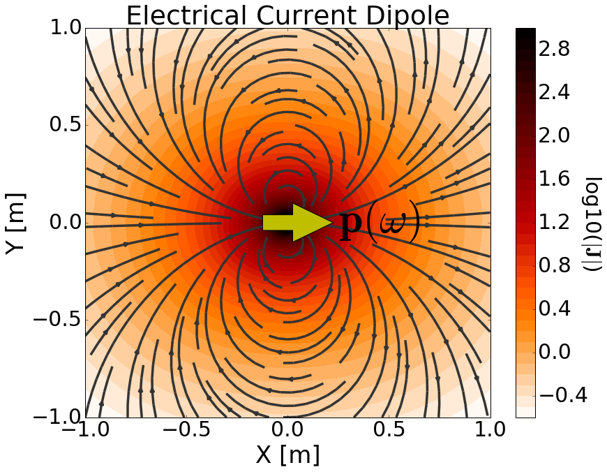
Fig. 65 Physical representation of the electrical current dipole source where \(\mathbf{p}\) = 1 Am.
The electrical current dipole can be thought of as an infinitesimally short length of wire which carries a current. The strength of the source is defined by its dipole moment (\(\mathbf{p}\)). This leads to an electrical source term of the form:
where \(\delta (x)\) is the Dirac delta function. The source is responsible for generating a primary current density (\(\mathbf{J}\)) in the surrounding region; secondary electric and magnetic fields are discussed later. This is illustrated in Fig. 65. In many cases, the term ‘electric dipole source’ is used instead. However, a true electric dipole represents the polarization of electrical charges of opposite sign.
Wire Model for an Electrical Current Dipole
In order to develop a more detailed definition for the electrical current dipole, let us first consider the source current from a wire of finite length. Assume the wire has length \(\Delta s\) and carries a current \(I\) which flows in the \(\mathbf{\hat x}\) direction along the wire. The source current density \(\mathbf{J_e^s}\) for the wire segment is given by:
where \(u(x)\) is the unit step function. In Maxwell’s equations, \(\mathbf{J_e (r)}\) defines the electrical source term and has units A/m \(\!^2\).
As we can see in Fig. 66, the source generates a primary current density (\(\mathbf{J}\)) in the surrounding region. Notice how the current flows out one end of the wire and into the other (Fig. 66 left). However, when the wire segment is much smaller than the scale of observation (\(\Delta s \ll r\)), then it appears as though the current density converges to a single point; see Fig. 66 (right). The purpose of the electrical current dipole is to approximate a finite wire segment when observation scales are much larger than the wire’s length. The electrical current dipole accomplishes this by defining a source term which exists at a single point in space.
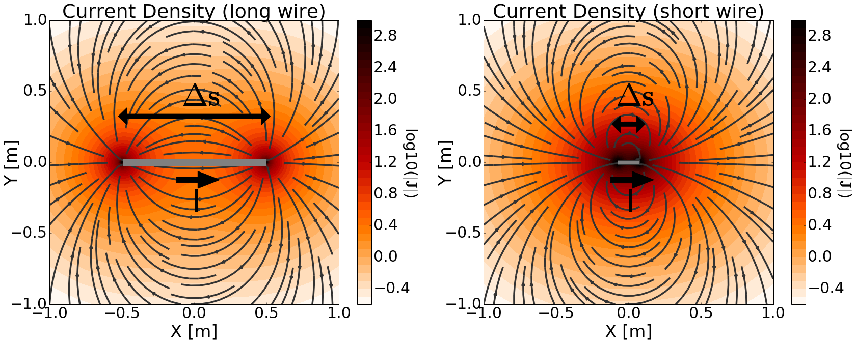
Fig. 66 Electrical current density due to a finite current-carrying wire. Long wire (left). Short wire (right). For both wires, the current was adjusted so that \(I\Delta s\) = 1 Am.
The electrical current dipole source is defined by letting \(\Delta s \rightarrow ds\) in the previous equation; making it a wire of infinitessimal length. As a result, the source current density for a harmonic electrical current dipole in the \(\mathbf{\hat x}\) direction is given by:
Fig. 67 Primary electrical current density due to an electrical current dipole with \(\mathbf{p}\) = 1 Am.
Examining Fig. 67, we see that the current density in the surrounding region converges to a single point; just like in Fig. 66 (right). However like a finite wire segment, the current still flows outwards from one side of the source and into the other.
If we consider an electrical current dipole oriented in an arbitrary direction, the source current becomes a vector \(\mathbf{I}\). Thus, the source current density for an electrical current dipole is given by:
The strength of the electrical current dipole source is defined by its dipole moment (\(\mathbf{p}\)). As we can see from the previous equation, the source term depends on the product \(\mathbf{I} ds\). Thus the dipole moment for an electrical current dipole source is given by:
where
From our definition of the electrical current dipole, \(\mathbf{p}\) has units Am, each of the Dirac delta functions carry units m \(\!^{-1}\), and thus \(\mathbf{J_e^s}\) has units A/m \(\!^2\).