Lessons Learned

We have learned the following two lessons from the HeliSAM survey and inversion at Lalor VMS deposit.

Warm-Start Inversion

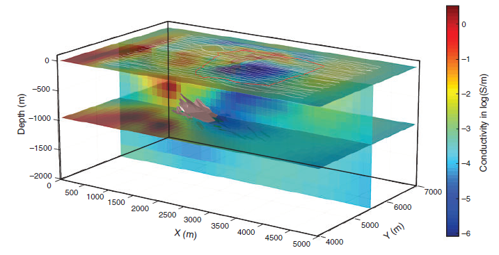
Fig. 442 Late-time inversion with a uniform half-space initial model results in an erroneous inversion result, in which the conductors are pushed the outside of the survey area.

It is a common practice to start an EM inversion with a uniform half-space assuming no existing structure in the model. However, at Lalor, we have found that a warm-start with two conductive blocks is necessary. When inverting the late-time data with a uniform half-space initial model, the inversion fits the observed data with an alternative model that is mathematically acceptable but geologically erroneous (Fig. 442).

Although the non-uniqueness of geophysical inversions is well-known, a complete failure like this is surprising in EM where there are supposed to be sufficient horizontal and depth resolution. Readers are referred to the original reference for the discussion on the plausible reasons.

Inversion for Near-Surface Infrastructure

The difficulty of inverting early-time data is from the fact that the 100-m cells originally designed for the geologic features are not small enough to capture the signature of the power line cable. So the mesh needs to be refined to a point that the coarseness of the mesh does not prevent the inversion from fitting the data. Here, we run three trial inversions of the early-time data with three different cell sizes (100 m, 50 m, and 25 m) around the power line area. The convergence curves of the trial inversions show that there is still significant amount of anomaly that cannot be fit by using the 100-m mesh, but the resolving powers of the 50-m and 25-m meshes are very similar (Fig. 443). It is then determined that a mesh refinement to 50 m would be sufficient in the inversion of early-time HeliSAM data at Lalor.

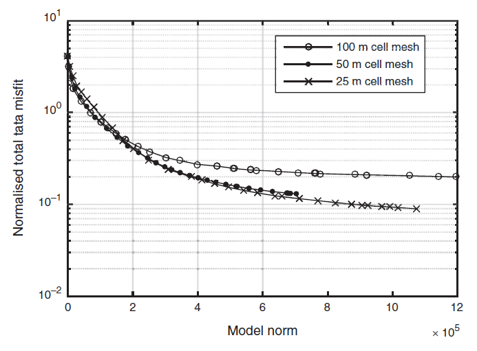
Fig. 443 The convergence curves of the three trial inversions using different cell sizes. The 50-m cell mesh and 25-m cell mesh perform similarly, so 50 m is deemed sufficient to capture the anomaly from the power line in the early-time data.

Another difficulty associated with the power line, if compared to a geological unit, is that the smooth constraints routinely used in the inversion is not suitable for the infrastructure, which is likely to have sharp interfaces. In this case study, we expect a large discontinuity between the cells for the power line and for the surrounding earth. Different methods can be used to recover sharper boundaries in a voxel inversion. Here, without altering the algorithm, we adopt an ‘iterative Tikhonov’ approach that uses an updated reference model for each step in the inversion. We take the recovered model from the 50 m cell mesh inversion, and isolate the conductive cells near the surface in the area where the infrastructure is expected. Then the inversion was started over again with a new reference model that consists of the near-surface power line cells embedded in a uniform half-space. Because the infrastructure is already in the reference model, their contrast with the surrounding is not subject to the penalty of smoothness.