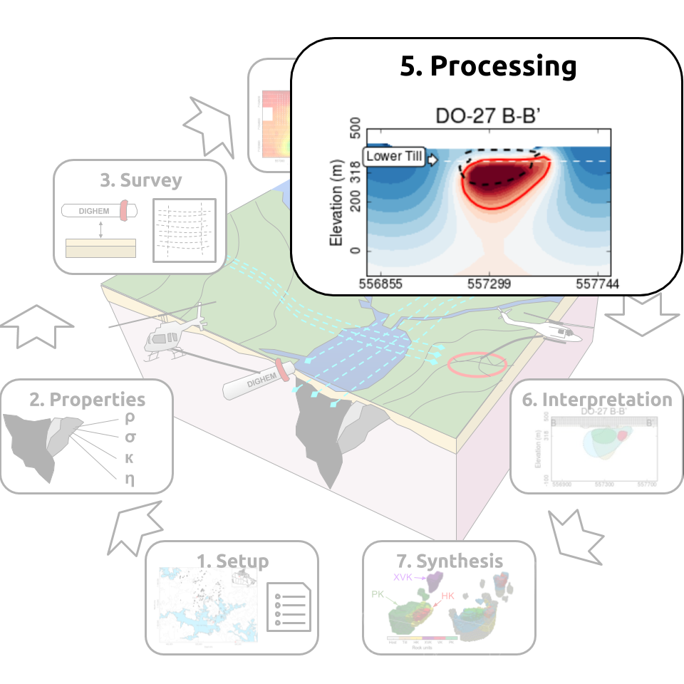
Processing

This section provides an overview of the data quality control and inversion procedure of the geophysical data.

Gravity

In preparation for the inversion, the following processing steps were taken on the ground gravity data:

• Since elevation information were only provided for the southern survey, the vertical position of the gravity stations were assigned using the topography model.

• The Bouguer-corrected data hovered around 1800 mGal, from which we subtracted a regional field of 1803.163 mGal.

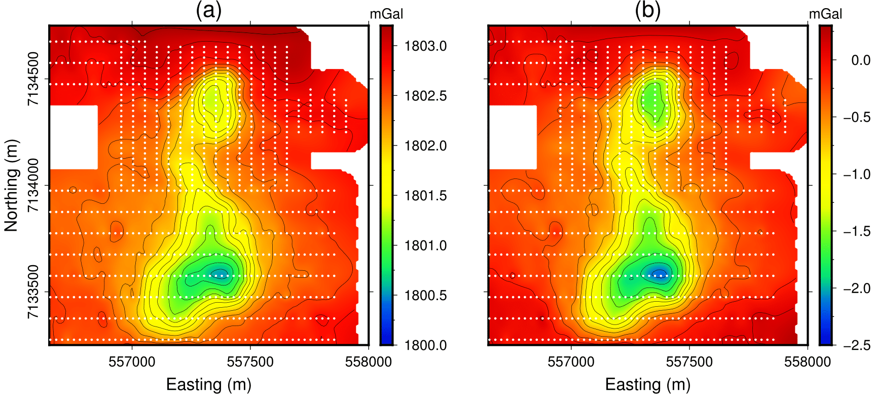
Fig. 371 Gravity data before and after leveling

Fig. 371 compares the gravity data before and after leveling. The processed data suggests a substantial negative density contrast in the area of the two pipes and a smaller negative contrast between them.

Data were then inverted with the UBC-GRAV3D inversion software. Uncertainty of 0.045 mGal were assigned to the gravity data. Inversion parameters for the mesh and regularization are presented below.

Number of cells	105 x 114 x 49
Core cell size	20 x 20 x 20
Regularization \([\alpha_s,\alpha_y,\alpha_x,\alpha_z]\)	1e-4, 1, 1, 1
Target chi factor (\(\phi_d^*\))	1.0

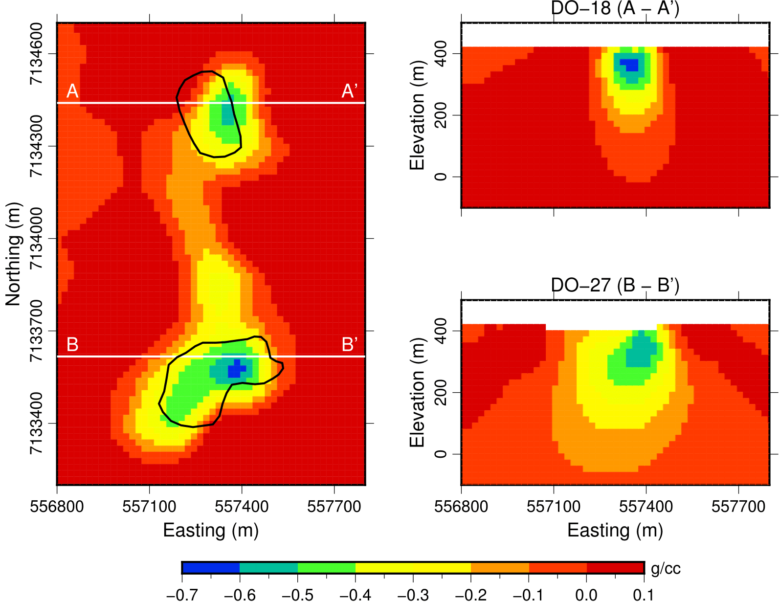
Fig. 372 Recovered density model.

Sections through the recovered density model are presented in Fig. 372. We note the following features:

• Two density lows near the location of the kimberlite pipes and extending at depth.

• A continuous density low is also observed between the two pipes but appears to be limited to roughly 75 m below topography.

Gravity Gradiometry

In preparation for the second density inversion, the following processing steps were taken on the airborne gravity gradient data:

• Data locations were converted from their native coordinate system (NAD83) to NAD27.

• The survey extent was reduced to the limits of the area of interest.

• Gradient data were leveled with a DC shift 2 Eotvos.

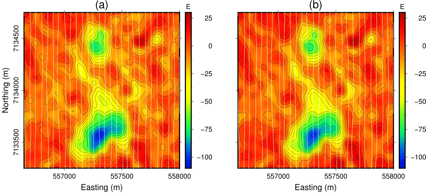
Fig. 373 Gravity gradient data before and after processing.

Fig. 373 compares the gravity data before and after processing.

Data were then inverted with the UBC-GG3D inversion software. An uncertainty value of 5 Eotvos was obtained by calculating the standard deviation of the west-most line of data, which was considered to be in the background and away from the kimberlites. The mesh contained 20 m and 10 m cells in the horizontal and vertical directions, respectively.

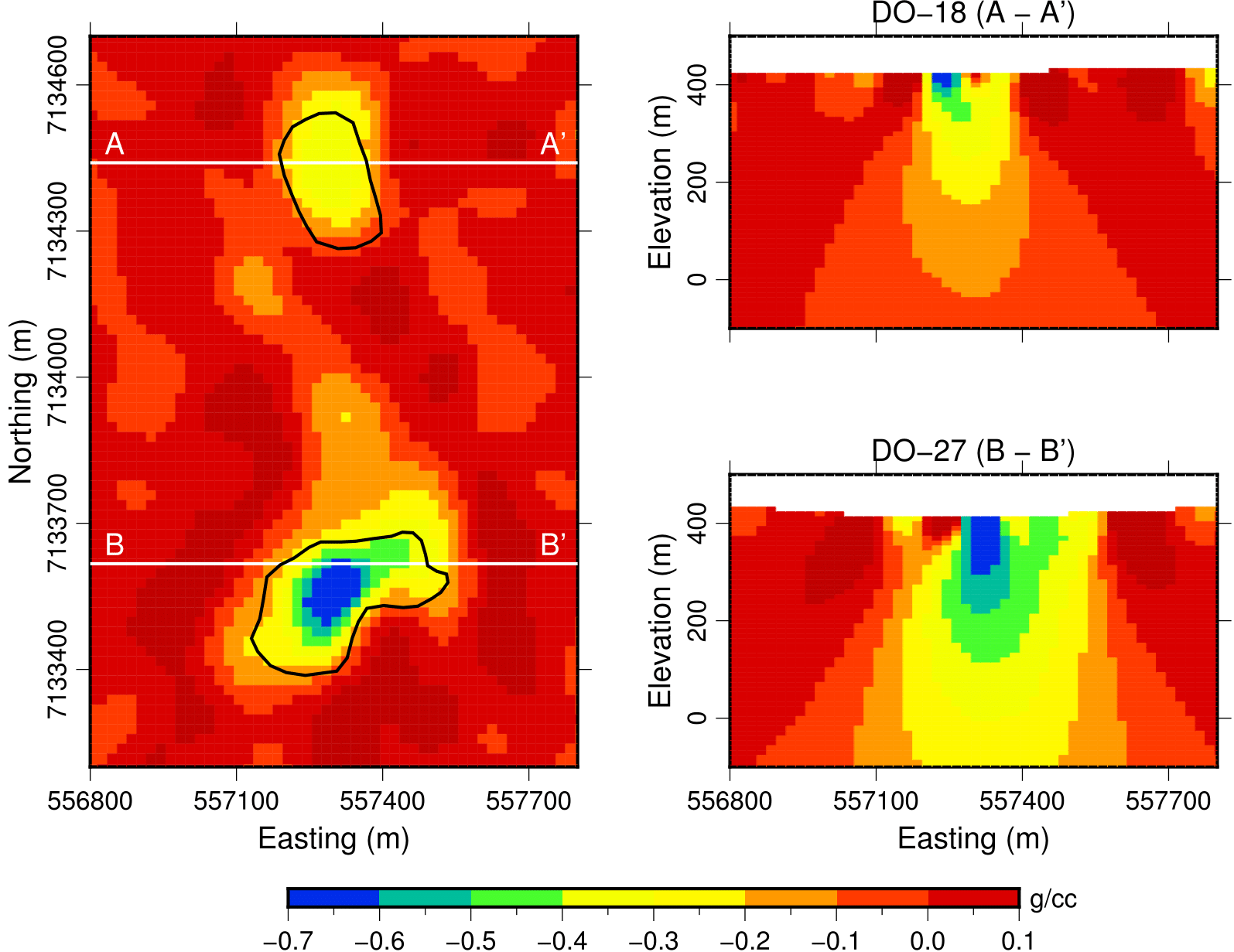
Fig. 374 Recovered density model from the gravity gradient data.

Sections through the recovered density model are presented in Fig. 374.

• Density anomalies are recovered directly at the location of the known kimberlite pipes conduit with low density material extending northwards from DO-27 (similar to that of the gravity result).

• The near surface fluctuations in density contrast can also be observed in the data.

Going forward

We have recovered two density models from the ground gravity and airborne gravity gradiometry. Two major challenges were faced in using the ground gravity data:

• The missing elevation over DO-18 had to be inferred.

• The center of the DO-18 anomaly differs by approximately 100 m from the known position of the pipe. This suggests that the two ground surveys may not have been stitched together accurately.

Going forward, we will focus on the airborne data set as we have more confidence in the accuracy of the gravity gradiometry data.

Magnetics

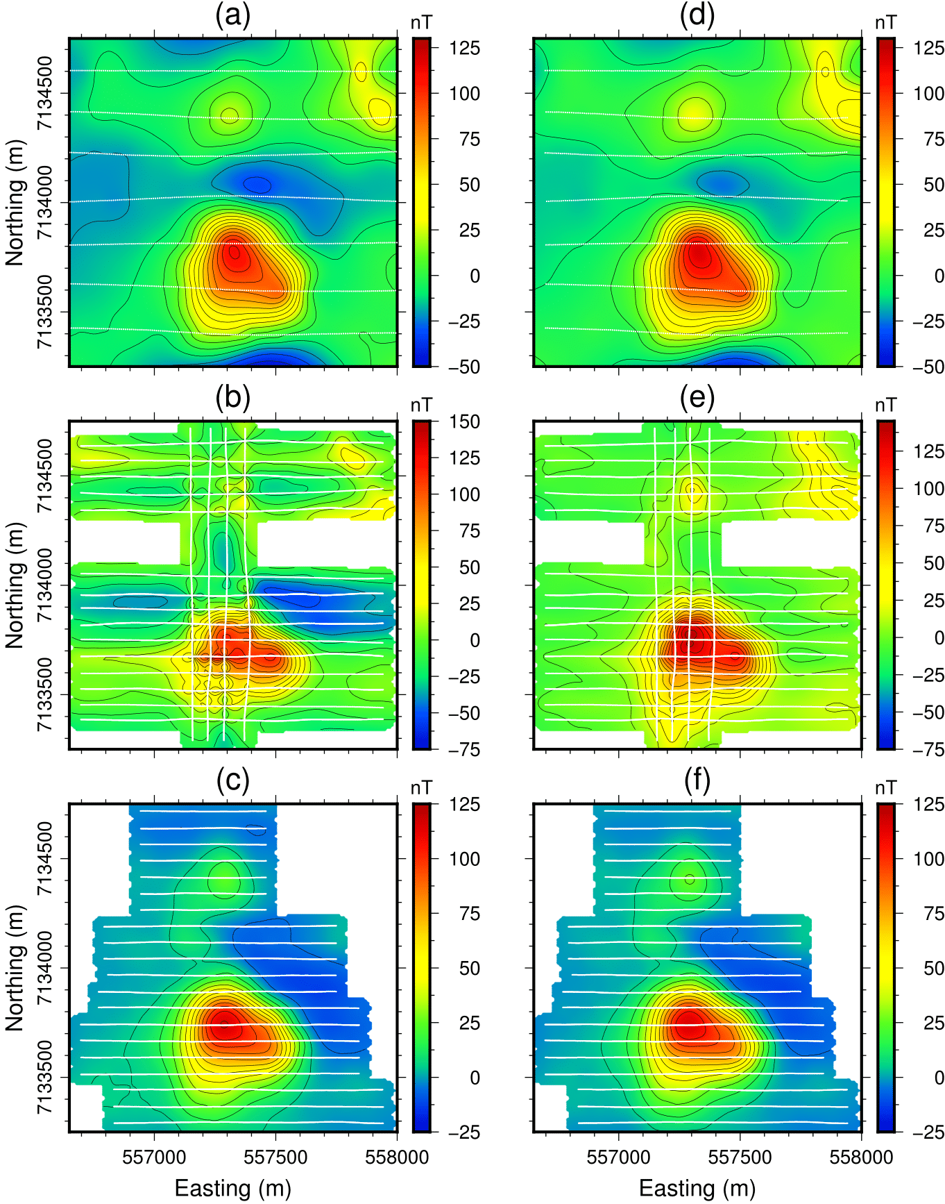
Fig. 375 Magnetic data before and after leveling.

We have three magnetic datasets collected with different instruments and at different times. Before inverting the data, we first proceeded with the following leveling steps:

• Data extent from the VTEM and DIGHEM surveys was reduced to the extent of the AeroTEM survey.

• We subtracted a constant from the DIGHEM and VTEM magnetic data such that the values away from the main anomalies were zero. The removal of a DC component was preferred over a polynomial fit because the latter can remove signal.

• In case of the AeroTEM magnetic data, it was noticed that each individual line had a varying DC shift. By comparing data points that have similar locations to those of the VTEM magnetic data, we were able to level each line in the AeroTEM magnetic data separately.

Fig. 375 compares each datasets before and after leveling. The peak magnetic anomalies measured over DO-27 are consistent across surveys. The signal from both DO-27 and DO-18 are now visible on the AeroTEM data set.

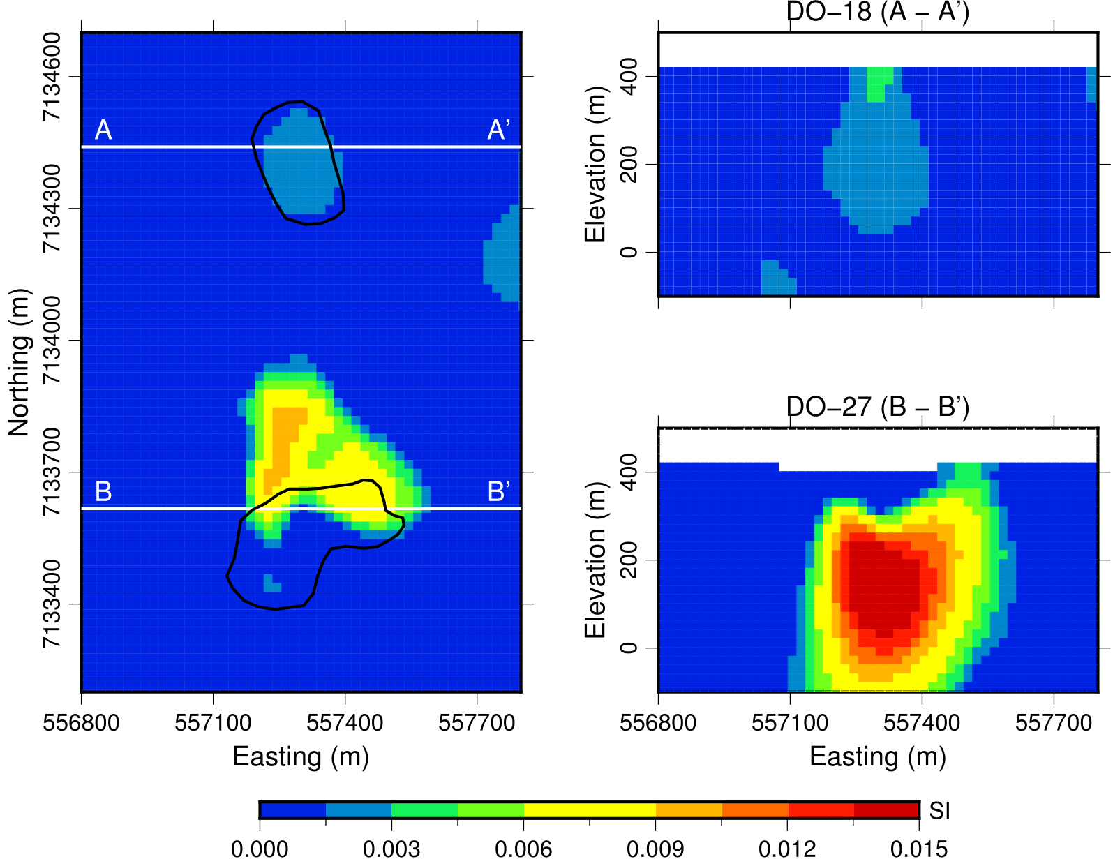
Fig. 376 Recovered susceptibility model from the VTEM magnetic data.

Despite the above leveling, the AeroTEM was still very noisy and difficult to invert. As well, the DIGHEM data were relatively sparse over the region of interest compared to the VTEM data. Overall, the VTEM data were the cleanest and provided the best coverage so we only present results from inverting the VTEM magnetic data, which was done with the UBC-MAG3D inversion software. We use the same mesh as for the density inversion. Sections through the recovered density model are presented in Fig. 376. We note the following:

• The largest susceptibilities are concentrated on the northeast edge of DO-27.

• Moderate to low susceptibilities are recovered at the center of DO-18 and at depth.

Frequency-Domain EM

1D Inversion

In preparation for a full 3D interpretation, we first inverted the FEM data in 1D. The 1D inversion assumes only vertical variations in conductivity, which greatly reduces the complexity and computational cost compared to a full 3D inversion. It can provide a first-order estimate for the background conductivity and validate the positioning, normalization and noise level associated with the data. We designed specifically for this project a Laterally Constrained 1D inversion strategy that uses the UBC-EM1DFM inversion algorithm as its central solver.

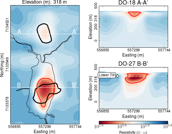
Fig. 377 Recovered conductivity model through laterally constrained 1D inversions.

Inversion parameters used for the 1D inversion are summarized below. Sections through the recovered conductivity model after convergence of the Laterally Constrained are presented in Fig. 377. The main features are:

• Conductivity highs mainly restricted to the upper 200 m below topography.

• Host Archean granitic rocks are highly resistive (\(2 \times 10^{4} \Omega \cdot m\)).

• The horizontal conductor near DO-18 seems to arc down in cross-section. This is likely due to the 1D representation of a compact 3D object.

Data type	(HCP) In-phase, Quadrature
Uncertainty	900 Hz	7,200 Hz	56 kHz
	1 nT	3 nT	5 nT
Number of stations	1153
Discretization	Depth	Cell Size
	0 < z < 40 m	2.5 m
	40 < z < 100 m	5 m
	100 < z < 400 m	10 m
Reference conductivity	\(5 \times 10^{-4}\) S/m

3D Inversion

Although the 1D inversion of the FEM data has yielded valuable information, the geometry of the TKC deposit is clearly 3D and hence a more sophisticated inversion algorithm is required. We use a tiled version of e3D_octree code, an inversion algorithm adapted from [Hab14]. The 3D inversion is computationally challenging and required additional processing steps:

• Data were sub-sampled at 400 m station spacing along survey lines, for a total of 216 stations.

• Pseudo-3D conductivity model obtained above was transfered to an octree mesh with 2 m cells.

• Data were converted from ppm to Total Field values.

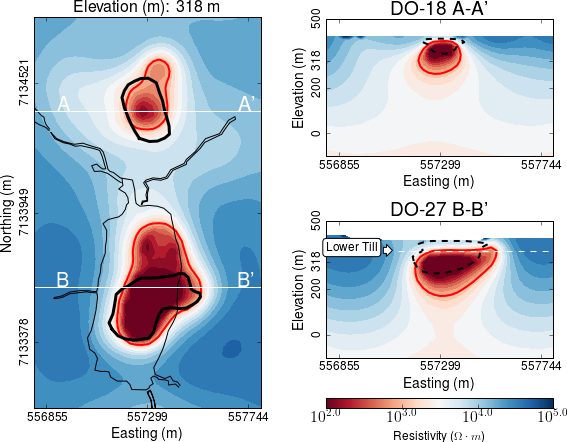
Fig. 378 Recovered conductivity model from 3D FEM inversion.

Fig. 378 presents sections through the recovered conductivity model. We note the following features:

• Both pipes show up as discrete and compact conductors extending vertically at depth.

• The conductivity structure associated with DO-18 appears to be close to the surface and the pipe is about 150 m in diameter.

• The upper limit of DO-27 is between 20 to 50 m below the lake; this is roughly the known thickness of till and lake bottom sediments [EB08].

While this upper limit seems well-defined by the inversion, the deeper limit of the pipe remains unclear. The bulk of high conductivity (\(>10^{-2}\) S/m) extends to at most 100 m below the till and the conductivity values gradually decrease below that. This may be a consequence of lack of resolving power by the survey. Our result does not exclude the possibility for a deeply rooted conductive pipe, for which the FEM is weakly sensitive.

Time-Domain EM

1D Inversion

We had access to AeroTEM II and VTEM surveys, but the AeroTEM II data were generally noisier away from the main EM anomalies. As a result, we choose to only invert the positive VTEM data. Using a similar strategy as implemented for the DIGHEM data, we first invert the VTEM data in 1D with lateral constraints using the UBC-EM1DTM inversion software. Since few of the time channels measured over DO-18 are positive, we focus our efforts on DO-27. We use the same mesh, starting conductivity and inversion parameters as for the FEM 1D inversion.

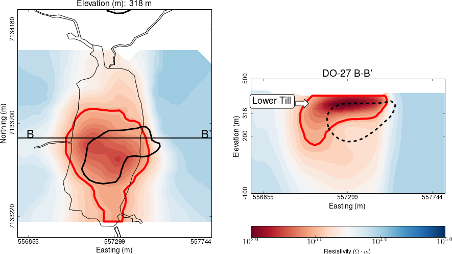
Fig. 379 Conductivity model from 1D laterally constrained inversions of TEM data.

Fig. 379 displays sections through the recovered conductivity model. The highest conductivity is centered at a depth corresponding to the interface between the till and the pipe below. The conductive anomaly extends to the surface and to depths of about 200 m.

To carry out the above analysis, we worked only with positive data. We note however that even the positive VTEM data at early times may still be contaminated with IP effects. Therefore, when trying to fit these decay curves in a voxel-based inversion code, these effects can manifest themselves as spurious artifacts, which may lead to erroneous interpretations. For this reason, we resorted to a cooperative inversion strategy.

Cooperative Inversion

We have so far inverted DIGHEM and VTEM data sets independently. While sensing the Earth differently, both EM systems are probing the same conductivity structure and should therefore agree on the general shape of the kimberlite pipe. In both cases, the horizontal location and vertical extent of the DO-27 kimberlite pipe are consistent. The pipe appears to extend to depths \(>\) 200 m below the surface. The two EM systems disagree however on the upper limit of the pipe.

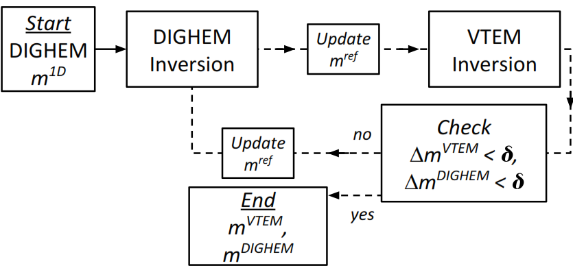
Fig. 380 Coopeerative inversion workflow.

To find a single conductivity structure that adequately explains the deposit, we re-invert both data sets with a cooperative inversion strategy [MO14]. Due to the limited coverage of the positive VTEM data, we limit the analysis to DO-27.

Fig. 381 gives a schematic representation of the cooperative inversion workflow. The DIGHEM data are inverted in 1D to get a general distribution and range of conductivity values. Since this model is already stored and interpolated in 3D, it is readily transfered to a different mesh to serve as a starting model for the 3D code. The outcome of the 3D DIGHEM inversion is then used as a reference model to guide the VTEM inversion. This iterative process is repeated until: (a) both data sets can be predicted within an acceptable level; and (b) the recovered models do not change substantially between each cycle (\(\Delta \mathbf{m} < \delta\)). Four iterations were carried out.

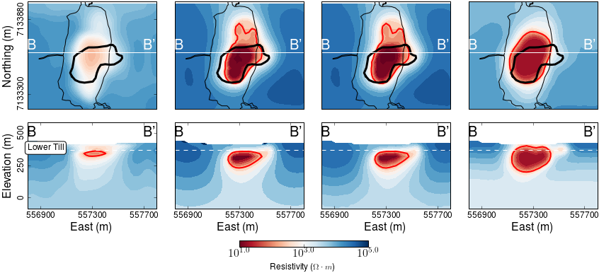
Fig. 381 A sequence of conductivity models through cooperative inversions.

Fig. 381 compares the sequence of inverted models. From left to right: (1) unconstrained FEM 1D inversion, (2) unconstrained FEM 3D inversion, (3) final cooperative FEM and (4) final cooperative TEM model.

IP Processing

Extracting chargeability information from airborne EM data is a field of active research. We follow TEM-IP inversion workflow developed by [KO16]. This workflow includes four steps:

1. Invert TEM data, and recover an estimated conductivity model, \(\sigma_{est}\), as shown in Fig. 381

2. Estimate the fundamental data, \(F[\sigma_{est}]\), and subtract them from \(d\); this generates raw IP data. This process is referred to as EM-decoupling.

3. Using a linear form of the IP response, invert the raw IP data at multiple times to recover pseudo-chargeability.

4. Finally, consider a single cell at which pseudo-chargeabilities at multiple times have been obtained. Use a Cole-Cole model [CC41] to parameterize time-dependent conductivity, and solve a small inverse problem to estimate: \(\eta\) and \(\tau\) with fixed \(c\) (either 1 or 0.5).

EM-Decoupling

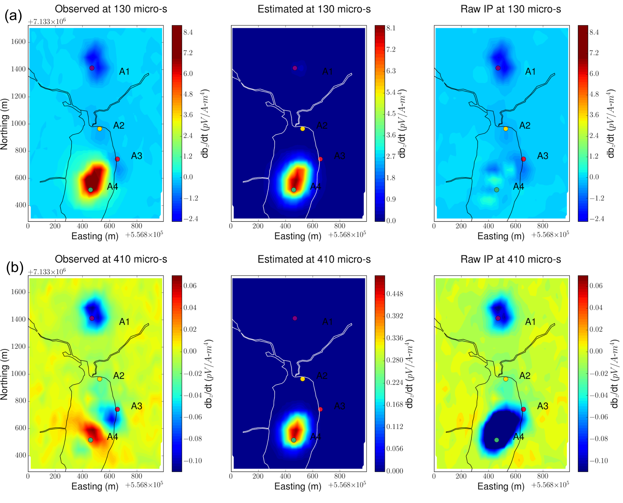
Fig. 382 EM-decoupling.

Fig. 382 illustrates how our EM decoupling is effective by concentrating on two times: 130 and 410 \(\mu s\), with plan view maps of \(d\), \(F[\sigma_{est}]\), and \(d^{IP}_{raw}\). At 130 \(\mu s\), near A4 we effectively removed the positive high anomaly (from the conductive DO-27 pipe) to reveal low amplitude IP features. Near A1-A3, the EM-decoupling results in stronger negatives. At 410 \(\mu s\), near A4, the EM-decoupling makes a greater impact, and it converts positive observations to large amplitude negative IP data.

IP Inversion

Having separated the EM and IP signals in the VTEM data, the obtained \(d^{IP}_{raw}\) at each time channel can now be inverted to recover a 3D pseudo-chargeability. The inversion is carried out for all time channels as described in [KO16].

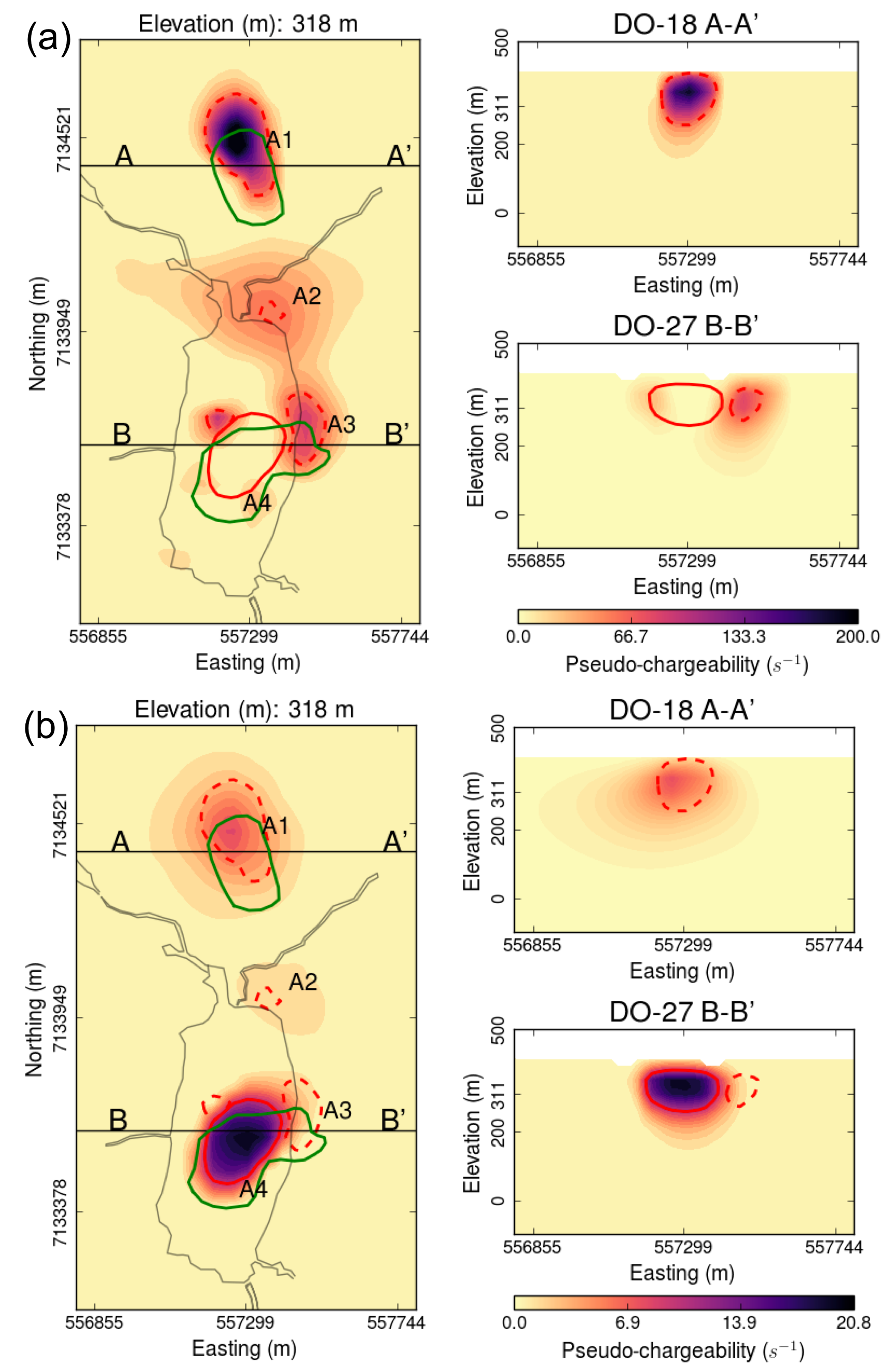
Fig. 383 Pseudo-chargeabilities at (a) early and (b) late times.

Fig. 383 presents the recovered pseudo- chargeabilities at two time channels: 130 and 410 \(\mu s\).

• Four chargeable bodies are imaged close to the four IP anomalies, A1-A4, that were previously recognized.

• At 130 \(\mu s\) three chargeable bodies close to A1, A2, and A3 are recovered, but none at A4 (DO-27).

• At 410 \(\mu s\), a chargeable body is imaged close to A4.

These distinct chargeable features reflect the different time decays associated with the IP signals: A1-A3 decay faster than A4.

Extracting intrinsic IP parameters

We have recovered a distribution of pseudo-chargeability values at multiple times and we now wish to use those results to extract intrinsic information about the polarization parameters of the kimberlites. We use a Cole- Cole model to characterize the complex conductivity in Laplace domain:

\(\sigma(s) = \sigma_{\infty} - \frac{\sigma_{\infty} \eta}{1+(1-\eta)(s\tau)^c}\)

where \(s=\imath\omega\) is a Laplace transfrom parameter, \(\sigma_{\infty}\) is conductivity at infinite frequency (S/m), \(\eta\) is chargeability, \(\tau\) is time constant (s), \(c\) is frequency dependency. In our analyses, \(\sigma_{\infty}\) and \(c\) are assumed to be known, hence we are only estimating the chargeability (\(\eta\)) and time constant (\(\tau\)) in the inversion.

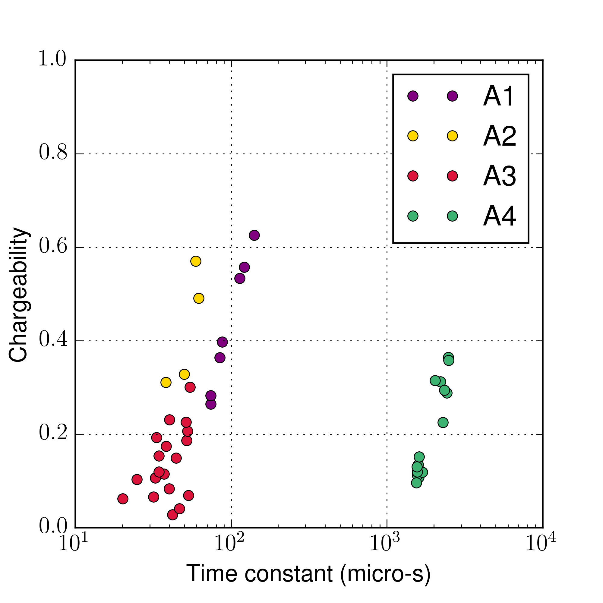
Fig. 384 Cross plots of recovered time constant and chargeability values.

Fig. 384 presents a cross-plot of the recovered chargeability (\(\eta\)) and time constant (\(\tau\)) for the cells close to A1-A4 anomalies.

• A4 can easily be distinguished from the others based on \(\tau\)

• A1 and A3 can be differentiated by \(\eta\) and perhaps by \(\tau\)

• The distinction between A1 and A2 is subtle, but it may be possible based upon \(\tau\) values