Processing and Interpretation
CSEM Data
In order to resolve the interpretation ambiguity inherent when only seismic data are considered, we used resistivity information derived from controlled source electromagnetic (CSEM) data. CSEM has been used successfully as an offshore hydrocarbon exploration tool for over a decade ([Con10]). The data for this study has been collected in a relatively new way; using a towed source and array of electric field receivers ([EMMD14, KDM+14]). MacGregor and Tomlinson ([MT14]) provides an overview to the offshore CSEM method and the various acquisition methods that can be applied.
The CSEM analysis was focused on line 5001. A 2.5D inversion approach, in which the earth structure is 2D and the source is a 3D point dipole, was therefore applied. Although this does not take into account the full 3D structure of the earth, in many circumstances it provides a good approximation to the resistivity structure along the line inverted. The effect of this approximation on the results is discussed in more detail below. Fig. 329 shows an example of the CSEM acquired along line 5001, in the form of source gathers at 1Hz. A significant response to the accumulation encountered at Wisting Central can be clearly seen in the CSEM data, particularly in the phase response (lower panel of Fig. 329 around 611km Easting). This is observed across a wide band of frequencies. It should be noted that it is somewhat unusual to see such a large reservoir response in the data directly. In this case the oil accumulation at Wisting is both extremely resistive (several thousand Ωm) and at a relatively shallow depth below mudline (about 300m) leading to the large response observed.
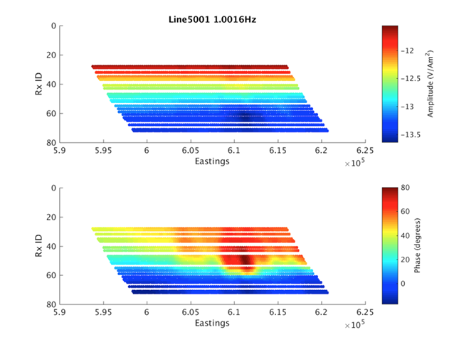
Fig. 329 CSEM Amplitude (top) and phase (bottom) data collected at 1Hz along line 5001. The effect of the oil accumulation at Wisting Central (around 611km Eastings) is clear, especially in the phase data.
The CSEM data for six frequencies (0.2Hz, 0.8Hz, 1Hz, 1.4Hz, 2.2Hz, 2.6Hz) were inverted using an Occam approach ([CPC87, KDM+14]) to derive anisotropic resistivity models that are smooth in a first derivative sense, and therefore as close to a uniform halfspace as possible, while honoring the data. A layered seawater conductivity structure based on measurements throughout the water column and 1D modeling was used. Nineteen to twenty-three source-receiver pairs per frequency were included in inversion.
The inversion was performed in stages. Firstly, an unconstrained inversion was run in order to examine the resistivity structure obtained in the absence of any a priori information. However unconstrained inversions in general have poor resolution. Resolution can be improved by including structural information from the seismic data. This also ensures consistency between seismic and CSEM derived results, which is important for subsequent integrated interpretation. Following unconstrained 2.5D inversion therefore, seismic data were used to condition the inversion of the CSEM data by adding structural constraint in the form of breaks in the smoothness requirement at selected seismic horizons, thereby improving the resolution of the CSEM result. Two versions of constrained inversion were run, one with a regularization break at reservoir level (top Stø ) only, and one with regularization breaks at both top Stø and the Intra-Snadd horizon. After initial constrained inversion testing, the resistivity was limited between 0.1 to 40 Ωm from seafloor to top Stø for both horizontal and vertical resistivity.
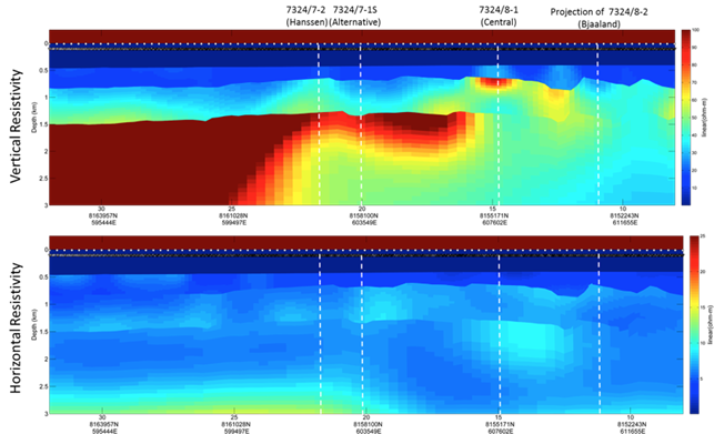
Fig. 330 Vertical resistivity (top) and horizontal resistivity (bottom) models recovered by 2.5D inversion for line 5001P1009 CSEM data. The inversion was constrained with regularization breaks at Top Stø and Intra Snadd. The Hanssen, Alternative, and Central well locations are marked by the white lines.
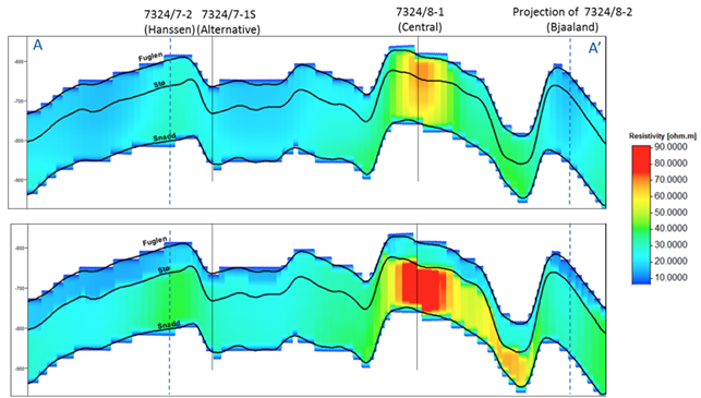
Fig. 331 Cross-sections along A-A’ (Figure 5) of CSEM-derived vertical resistivity for (top) unconstrained inversion, and (bottom) inversion constrained by the top Stø horizon and Intra-Snadd horizon. The Intra-Snadd horizon (a deeper horizon that is outside the area of interest for the remainder of the analysis not shown in the Figure) is about 500 m. deeper than the Snadd horizon.
Fig. 330 shows the vertical (upper panel) and horizontal (lower panel) resistivity resulting from the final constrained inversion that were carried using depth- converted seismic horizons top Stø horizon and Intra-Snadd horizon.
Background resistivity is extremely high in the area with vertical resistivity of 25-30 Ωm. Background anisotropy is also extremely high with factors of five or more observed. This high overburden resistivity and anisotropy is the result of the significant uplift in the area. A significant increase in vertical resistivity was recovered in the lower Snadd, with localized variations contained within a regional feature. This regional feature also exhibits extremely high electrical anisotropy.
A localized resistive feature coincident with the structure penetrated at Wisting Central is clearly recovered in the vertical resistivity. A more subtle increase in resistivity is observed at the Hanssen well location. No localized resistive feature is recovered in the Stø at the location of the Wisting Alternative or Bjaaland wells.
Fig. 341 shows the CSEM-derived vertical resistivity in the same windows of analysis used in the seismic quantitative interpretation, for the unconstrained and constrained inversions run: The top one corresponding to the unconstrained inversion, and the bottom image shows the results of the constrained inversion previously shown in the Fig. 330.
A qualitative interpretation of the CSEM inversion results supports the outcome of the Alternative, Central and Bjaaland wells. A prominent resistivity anomaly is recovered at Central, in which there was a significant oil discovery, which is in agreement with the high resistivity values measured at the reservoir location. On the other hand, the Realgrunnen structures penetrated at Alternative and Bjaaland, two dry wells, are related to low resistivity values that support the petrophysical outcome. At the location of the Hanssen discovery well, a subtle high resistivity anomaly is observed. The relatively small magnitude of this feature is the product of a 3D effect in the CSEM data, a consequence of the location of the CSEM line with respect to the location and the size of the reservoir (see Fig. 322 b). Although in many circumstances the 2.5D approximation is a good one, if the resistive reservoir is relatively small, or the 2D line being inverted is close to the edge of the reservoir, then the effect of the of the reservoir on the CSEM data is diminished, and consequently the resistivity recovered by a 2.5D inversion is reduced from its true value. Loseth et al. illustrate this with a synthetic modelling study in which they demonstrate the reduction in inverted resistivity with width of the target reservoir and proximity of the CSEM line to the reservoir edge. In the case of Hanssen, the reservoir is both relatively small and the line is close to the edge of the body, leading to the lower resistivity at this location. The effect of this on the quantitative interpretation is discussed in later sections.
Seismic Data
The ultimate quality of any inversion depends on the quality of the input data, and to ensure a robust result, data must be optimally conditioned for the workflow to be applied. In this example, the input seismic offset gathers were pre-conditioned prior to inversion to increase the overall signal-to- noise ratio and avoid any remaining noise having a high impact on the inversion results. The pre-conditioning also corrected for offset dependent frequency loss and ensured that the gathers were aligned. Since data pre- conditioning, if not applied carefully, could significantly affect AVO behavior of target reflectors, the sensitivity of inversion results to the pre-conditioning approaches applied has been thoroughly tested and analyzed. It is important to note that all conditioning steps were parameterized keeping in mind the need to preserve amplitude behavior, and the minimum possible pre- conditioning was undertaken. The processes applied are summarized in [Sin09].
During the pre-stack seismic inversion, a global objective function is minimized in order to compute an optimal model for P- and S-impedance, which best explains the input angle stacks and is consistent with the geological knowledge introduced through a priori information ([TMR01]). Initial low frequency, models of P- and S-impedance were created based on seismic velocity and well data. These models exclude any reservoir signature and mix the lateral variations from the velocity field and vertical resolution from wells logs filtered at 5Hz. Wavelets were extracted per angle stack per well and later combined to obtain the most representative wavelet for each angle stack. Additional parameters such as scale factor between wavelets and actual amplitude sections, confidence in seismic amplitude angle stack data, number of iterations and allowed low frequency model standard deviations were also customized based on iterative tests performed per set of lines. Final results were then extracted along well trajectories and compared to actual well log data in order to ensure a good representation of the earth model. Also, percentage of differences between input and synthetic angle stacks were calculated to ensure that they were less than 20% of the original seismic amplitude. In this case, where the P- and S-impedance models were allowed to change 2000 [m/s gr/cc] from the initial model, after 25 iterations, the seismic inversion results represent very well both the earth model from the well log data and the actual partial angle stacks. (Fig. 332)
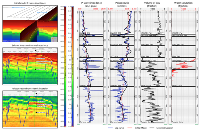
Fig. 332 Initial model, P-wave impedance and Poisson ratio from seismic inversion (left), tracks of P-wave impedance, Poisson ratio, volume of clay and water saturation extracted along the projection of the well 7324/8-1 (right).
The multi-attribute rotation scheme (MARS) ([ABolivarDiLucaS15]), was used to estimate rock properties and facies volumes from well log and seismic inversion attributes. This workflow uses a numerical solution to estimate a transform to predict petrophysical properties from elastic attributes. The transform is computed from well log-derived elastic attributes and petrophysical properties, and posteriorly applied to seismically-derived elastic attributes. MARS estimates a new attribute, t, in the direction of maximum change of a target property in an n-dimensional Euclidean space formed by n attributes. The method sequentially searches for the maximum correlation between the target property and all of the possible attributes that can be estimated via an axis rotation of the basis that forms the aforementioned space.
Multiple elastic attributes such as P-wave impedance \(Ip\), S-wave impedance \(Is\), P-to-S velocity ratio (\(Vp ∕ Vs\)), the product of density and Lamé’s parameters \(\lambda \rho\) and \(\mu \rho\) (Goodway et al., 1997), Poisson’s ratio \(\sigma\), the product of density by bulk modulus \(\kappa \rho\), the product of density and dynamic Young’s modulus \(E \rho\), Poisson dampening factor (\(PDF\)) ([Maz07]), etc., can be used in the MARS assessment. For this case study, for each target petrophysical property, MARS was run for a 2D combination of the 64 elastic attributes shown in Fig. 333 , which can be derived from \(Ip\) and \(Is\), resulting in the evaluation of 2016 independent bi-dimensional spaces. In this table, each number represents a single attribute, which is obtained after applying the mathematical operation shown in the leftmost column to the elastic attribute shown in the uppermost row. For example, the number 21 represents the attribute. The purpose of applying a mathematical operation (such as square root, power, inverse, logarithm, etc.) to attributes is to be able to model physical phenomena that exhibit nonlinear behavior. This is a mathematical strategy to linearize potential nonlinear relationship between the elastic attributes and the petrophysical properties, used with the goal of improving the correlation between the attribute t and the target petrophysical property.
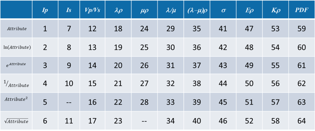
Fig. 333 Matrix of attributes used in MARS. Each number represents a single attribute, which is obtained after applying the mathematical operation show in the leftmost column to the uppermost row. For example, the number 21 represents the attribute.
The MARS approach was applied in two different depth windows, given the different rock physics relationships between the elastic attributes and the petrophysical properties in the Stø and Nordmela Fms. (see Fig. 324). The first window comprises the Fuglen and Stø Formations and the second window the Nordmela Formation. The rock properties that were estimated using the MARS approach were total porosity (\(\phi_T\)), volume of clay (\(Vclay\)) and the hybrid petrophysical property water saturation plus volume of clay (\(Sw+Vclay\)).
This last property, which can take values between zero and two, was used as input to build a litho-fluid facies volume based on the cut-off values shows in Fig. 334. Three litho-fluid facies were defined. The green facies denotes zones where clean hydrocarbon bearing sands with thickness above seismic resolution are expected to be found, including both commercial and residual saturation given the inability of the elastic measurements to distinguish between these two. The blue facies represents clean wet sand or shaly hydrocarbon bearing sand or thin hydrocarbon bearing sand that cannot be resolved at seismic resolution. These three configurations of rock and fluid present a high degree of overlap in the elastic domain, in consequence cannot be separated using seismic data. The last litho-fluid facies (brown) represents the background trend that are composed of shales or thin wet sand.
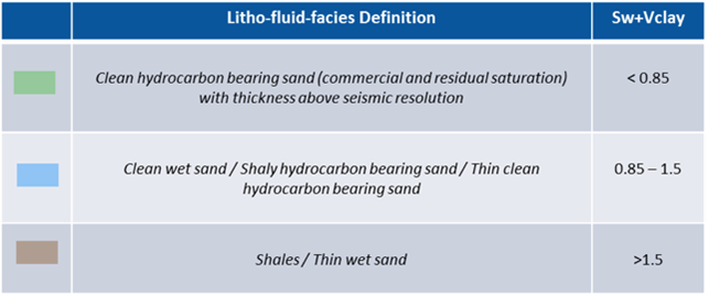
Fig. 334 Litho-fluid facies definition based on the hybrid petrophysical property \(Sw+Vclay\).
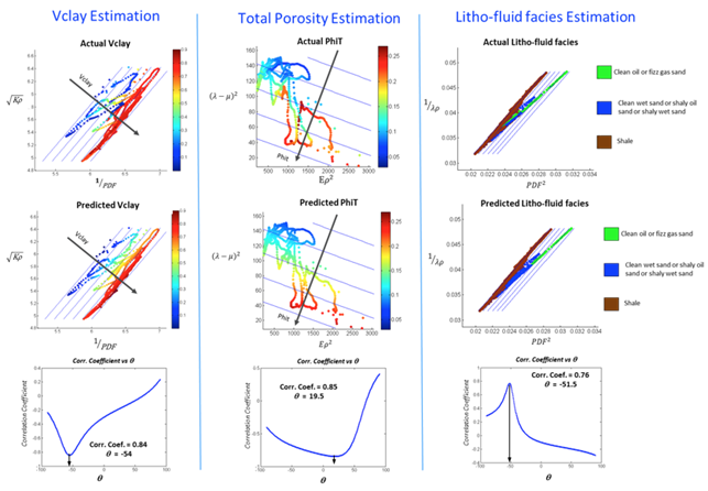
Fig. 335 Comparison of the actual (upper) and predicted (middle) target property log upscaled to seismic resolution for the Central and Alternative wells in the optimal cross-plot space estimated from the MARS analysis for the Fuglen and Stø Formation. Gray arrows, orthogonal to the blue lines, indicate the direction of maximum change of target petrophysical property in the optimal attribute space. The lower plots show a crossplot of the correlation coefficients between the target property log and the set of attributes estimated via axis rotation, versus the rotation angle (\(q\)). The black arrow highlights the angle where the maximum cross correlation was found.
The results obtained after applying MARS to well log information from the Central and Alternative wells is shown in Fig. 335 for the Fuglen and Stø Formations and Fig. 336 for the Nordmela Formation. These plots show a comparison between the actual and predicted target petrophysical property using MARS in the optimal elastic attribute space determined by a global search algorithm. The lower plots show a crossplot of the correlation coefficient between the derived set of attributes (estimated via axis rotation) and the target petrophysical log, versus the angle of rotation (\(\theta\)). These plots show for all the cases a fair to good maximum cross correlation that supports the application of the MARS-derived transform to seismically-derived elastic attributes to estimate sections of the target petrophysical properties along the 2D seismic lines analyzed.
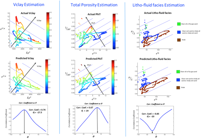
Fig. 336 Comparison of the actual (upper) and predicted (middle) target property log upscaled to seismic resolution for the Central and Alternative wells in the optimal cross-plot space estimated from the MARS analysis for the Nordmela Formation. Gray arrows, orthogonal to the blue lines, indicate the direction of maximum change of target petrophysical property in the optimal attribute space. The lower plots show a crossplot of the correlation coefficients between target property log and the set of attributes estimated via axis rotation, versus the rotation angle (\(q\)). The black arrow highlights the angle where the maximum cross correlation was found.
Once the transform to predict petrophysical properties from elastic attributes was found for each window using well log data, the resulting relationships were applied over the seismically-derived elastic attributes per window using the seismic horizons (upper window: from top Fuglen to base Stø, and bottom window: from base Stø to top Snadd), with the goal of estimating a single 2D section of total porosity, clay content and litho-fluid facies per 2D seismic line. The litho-fluid facies section was estimated after applying the cut-off presented in Table 3 to the seismically-derived section of \(Sw+Vclay\). The resultant litho-fluid facies, clay content and total porosity sections for the line 5001P1009, along with the corresponding well log information for the Central and Alternative wells is shown in Fig. 337. Notice the good match between the seismic and well log-derived petrophysical property in the calibration wells demonstrating that both were correctly predicted. In addition, the well trajectory of the Hanssen and Bjaaland wells are also shown (no log information is available for these wells). The former was catalogued as a discovery well and the latter as a dry well. The litho-fluid facies section suggests that hydrocarbon fluid is present in both locations, and highlights the fact that seismic data alone cannot distinguish between commercial and non-commercial hydrocarbon saturations, leaving a significant ambiguity in prospect de-risking.
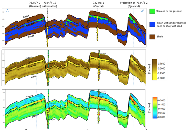
Fig. 337 For line 5001P1009, sections along A-A’ (Fig. 322) of litho-fluid facies (top), clay content (middle) and total porosity (bottom) along wells Central and Alternative derived from MARS analysis of elastic attributes. The curves overlaid in the top panel are \(Vclay\) (left) and \(Sw\) (right) and in the middle and bottom panels are volume of clay (left) and total porosity (right).
Interpretation
The final stage of the workflow is to combine the seismically derived properties, with the electrical information derived from the CSEM data. The goal of this stage is to reduce the uncertainty in fluid saturation that is observed in the seismic-only results. In order to do this, electric and elastic properties must be combined in a common domain and at a common scale so that direct comparison, and ultimately quantitative integration is possible.
Seismically-derived resistivity estimation and transverse resistance (TR) calibration
In order to allow direct comparison between seismic and CSEM results, the next step in the methodology (Fig. 320) is the estimation of resistivity models from seismically derived properties for different fluid saturation scenarios. With this goal in mind, we used the seismically-derived litho-fluid facies, clay content and total porosity sections with a calibrated rock physics model to transform these petrophysical properties into the electrical domain. The calibrated rock physics model used was the Simandoux equation ([Sim63]):
where
Parameters within the Simandoux equation were defined in the properties section. This rock physics model represents the same one used in the petrophysical evaluation of the Central and Alternative wells to estimate water saturation (\(Sw\)) from the horizontal resistivity log and was calibrated in the early stage of the study. The procedure used to estimate the seismically-derived resistivity sections at different fluid scenarios consisted of applying directly Eqs. (501) and (502) to the total porosity and volume of clay sections (Fig. 337) for different values of \(Sw\) that were modified only in those areas were the seismic indicates the presence of clean hydrocarbon bearing sand, i.e. green facies in the litho-fluid facies section (Fig. 337). The results are shown in Fig. 338 b, c, and d, for values of \(Sw\) equal to 0.1, 0.5 and 1 respectively. As a quality control of the results for the case of \(Sw\) = 0.1 (90% hydrocarbon saturation, which is a saturation close to that obtained from the petrophysical evaluation at the Central well), the measured resistivity curve was overlaid. An excellent match with the modeled resistivity is obtained. One important observation that can be made from the comparison of the three seismically-derived results is the low resistivity contrasts between the reservoir and non-reservoir facies for the case of \(Sw\) = 0.5. This demonstrates that this level of water saturation (or higher) cannot be identified using CSEM data in this particular geological setting due to the high values of the background resistivity.
At this stage in the workflow, results have all been transformed to the electrical domain. However, there is one further step required before a direct comparison can be made. It is noticeable that the seismic results in Fig. 338 are significantly higher resolution than the CSEM results in Fig. 338, even when the CSEM inversion is constrained. This difference must be resolved before the results can be compared or combined in a quantitative fashion.
The simplest approach to achieving this is to upscale both seismic and CSEM results. The reservoir parameter that is best constrained by the CSEM method is the transverse resistance (vertically integrated resistivity). By calculating the transverse resistance from the seismically and CSEM derive resistivity, the difference in vertical resolution between the two methods can be overcome, albeit at the expense of the higher resolution of the seismic result. Transverse resistances based on CSEM and seismic results are compared in Fig. 338 a. Note that when the resistivity is calculated from the seismic data using the Simandoux relationship, which is calibrated to horizontal resistivity at the well, the result is most closely related to the horizontal resistivity of the sub- surface. The CSEM measurements, in contrast, provide a measure of both horizontal and vertical resistivity however reservoir related structure manifests in the vertical resistivity. To address this difference, an empirical calibration factor of three, based on CSEM analysis of background anisotropy, was applied to the seismically derived transverse resistance to compensate for the electrical anisotropy observed.
An analysis of Fig. 338 a offers important information about the hydrocarbon saturation levels of the reservoirs and potential reservoirs along the section. A good agreement is seen between the CSEM and seismic transverse resistance curves at the end member positions represented by the Central well location (\(Sw\) = 0.1 - magenta curve) and for the Alternative well location (\(Sw\) = 1 - blue curve) that corroborate the validity of the rock physics model used and the calibration factor applied to the data. For the case of the Bjaaland well, the CSEM derived transverse resistance most closely agrees with the lower saturation seismically derived curves, indicating, in a semi-quantitative way, the absence of a commercial hydrocarbon saturation at this location. Finally, for the Hanssen well, the separation between the CSEM transverse resistance curve and that for the wet case seismically-derived curve (blue curve) indicates the presence of hydrocarbon saturation at least higher than 50%. However, it is important to have in mind that a diminished CSEM-derived resistivity value is expected to be found in this area due to the 3D effects discussed previously. As a consequence of this the hydrocarbon saturation will be underestimated in this case.
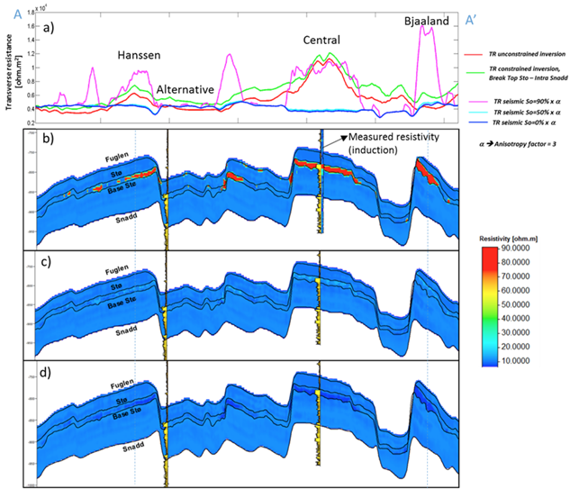
Fig. 338 (a) Comparison between the seismically- and CSEM-derived transverse resistance estimates. (b) Cross-section along A-A’ (Fig. 322) of seismically-derived resistivity for \(Sw\) = 0.1. (c) Same cross-section along A-A’ for \(Sw\) = 0.5. (d) Same cross-section along A-A’ for \(Sw\) = 1. Note the good match between the measured and modeled resistivity in the Central well at the (b) section.
Water Saturation Prediction
Although the semi-quantitative comparison of transverse resistance presented above provides valuable information on reservoir properties, it is often desirable to derive a quantitative estimate of rock and fluid properties. The last step in the workflow (Fig. 320), is therefore the quantitative prediction of the \(Sw\). The input data for this analysis was the seismically-derived porosity, clay content and litho- fluid facies section shown in Fig. 337, and CSEM-derived transverse resistance along the CSEM line (Fig. 338 a). These datasets were inverted using the Simandoux equation calibrated at the Central and Alternative wells, and a global search inversion method. This method seeks the value of \(Sw\) that provides the minimum misfit between seismically and CSEM derived transverse resistance, using a grid search algorithm (see Fig. 339). It is important to mention that only potential reservoir rocks as indicated by the seismic litho-fluid facies (green facies in Fig. 337 to the top), were considered to have variable \(Sw\) during the inversion process. In this way the quantitative seismic interpretation result not only provides information about the clay content and total porosity of the rocks, necessary for the Simandoux equation, but also about the location and thickness of the potential pay sand, thus maintaining seismic resolution in the final result. However, note that since only \(Sw\) varies during the inversion, it is implicitly assumed that the porosity and \(Vclay\) as defined by the seismic data are correct.
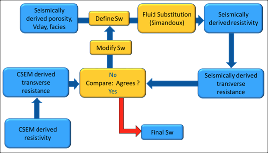
Fig. 339 Methodology used to estimate \(Sw\) from seismically-derived rock properties volumes and CSEM derived resistivity.
The result of this inversion is shown in Fig. 340. The top panel shows the profile of the misfit obtained as a function of the \(Sw\). This information can be interpreted as a measurement of the robustness of the \(Sw\) estimation. The middle panel shows how the optimal \(Sw\) is linked to the lowest misfit value. Note that in areas where no hydrocarbons are indicated by the seismic litho-fluid classification shown in the bottom panel for reference (i.e. outside the green facies), \(Sw\) is set to 1. Around Wisting Central, the inversion result shows a well constrained low \(Sw\) value, with a narrow inversion minimum. This is as expected since at low water saturations, a small change in \(Sw\) results in a relatively large change in resistivity. Around the Hanssen well, the inversion minimum is wider, a result of the lower predicted saturation. At Bjaaland, the results predict a minimum water saturation of about 50%, consistent with the sensitivity limit suggested by well log analysis.
Finally, the resulting \(Sw\) profile was mapped back in its correct position using the seismically-derived litho-fluid facies volume to generate a hydrocarbon saturation section along the line (Fig. 341). Excellent correlation with known well results was achieved. The integration of seismic, CSEM, and well data predicts very high hydrocarbon saturations at Wisting Central, consistent with the findings of the well. The slightly lower saturation at Hanssen is related to 3D effects in the CSEM data, but the outcome of the well is predicted correctly. There is no significant saturation at Wisting Alternative, again consistent with the findings of the well. At Bjaaland, although the seismic indicate the presence of hydrocarbon bearing sands, the integrated interpretation result again predicts correctly that this well was unsuccessful.
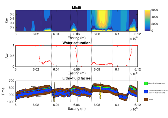
Fig. 340 Misfit as a function of \(Sw\) between the CSEM-derived transverse resistance and the set of seismically-derived transverse resistance computed for different \(Sw\) values (top). Optimal \(Sw\) estimation linked to the minimum misfit value (middle). Cross-sections along A-A’ (Fig. 322) of seismically-derived litho-fluid facies (bottom)
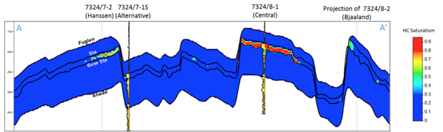
Fig. 341 Cross-sections along A-A’ (Fig. 322) of hydrocarbon saturation obtained from a joint interpretation of CSEM, seismic and well log data, with hydrocarbon saturation curves overlaid. Notice that the seismic data alone cannot distinguish between commercial and non-commercial hydrocarbon saturation. The inclusion of the CSEM resistivity information within the inversion approach allows for the separation of these two possible scenarios.