Processing

After data collection the raw data was processed in the Aarhus Workbench to remove noise. Coupled data arising from man-made installations such as buildings, power lines, cables, roads and railroads was also removed. Fig. 478 shows the data before (Fig. 478 a) and after removal of data affected by noise and couplings (Fig. 478 b).

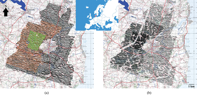
Fig. 478 Data soundings (a) before removal of data affected by noise and couplings and (b) after culling the coupled and noisy data.

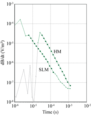
Fig. 479 Sounding curve.

The average flight speed of the entire survey was approximately 100 km/h or 28 metres per second. The average flight height for the transmitter frame was 30 metres above ground level. Typically, a repetition frequency of one full measure¬ment every half second is used, thus, with a flight speed of 28 metres per second the lateral distance between the raw data sets is approx¬imately 14 metres. Raw data is stacked during processing to enhance the signal-to-noise relationship, and in reality the resolution is 25-50 metres horizontally and less than a few metres vertically. Fig. 479 shows a db/dt sounding curve from the survey with LM and HM curves. The circles indicate the times that are actually used for interpretation of the data.

After initial processing, the data is interpreted using an interpretation algorithm implemented in the Aarhus Workbench software yielding a quasi 3D model of the resistivity of the subsurface down to 100 metres below ground level. Subsequently the geophysical models are presented as average resistivity maps at various elevation or depth intervals (Fig. 480) or in profiles (Fig. 481).

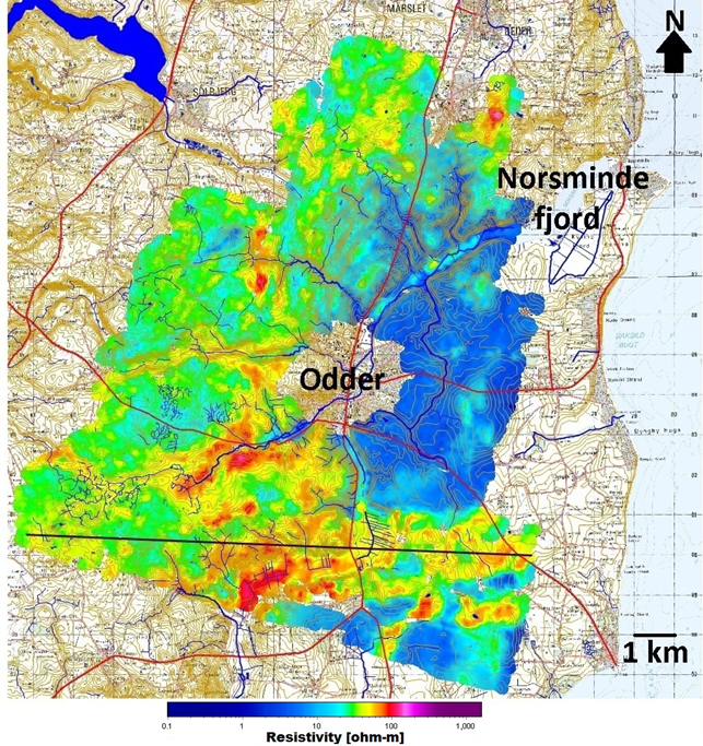
Fig. 480 The mid resistivity map for a depth of 15-20 metres. The position of the profile in Fig. 481 is marked in a black line. The map also shows the contours, in many places with a direct correlation with the geology.

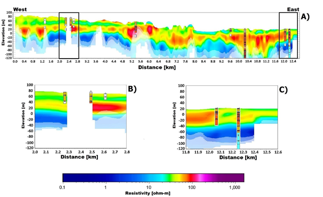
Fig. 481 Resistivity profiles. (a) Profile along line in Fig. 480. (b) and (c) are zoomed in profiles from (a).