Survey

It is expected that the mineralization is both conductive and chargeable. A DC/IP survey is therefore an appropriate (and desired) choice for geophysical exploration. In this section, we explore the survey design used at the Cluny property.

DC Resistivity (DCR)

The fundamentals for a DCR survey can be found in the Geophysical Surveys section. Many choices are possible for electrode layouts, but the final choice at Cluny was motivated by the following factors:

1. MIM, the company who was exploring the property, had developed their own data acquisition system MIMDAS. The system had a 100-channel capacity distributed acquisition system and each electrode could serve as a current or potential electrode. Both DCR and IP data can be acquired.

2. The area of interest is approximately 2 km by 5 km. Although full 3D coverage was desirable, the field acquisition was limited to 10 east-west lines. The reason for this was two-fold. Firstly, the 2D lines could be laid out across the East-West boundaries of Cluny region. Secondly, the fault structures were known to strike north-south, so it is natural to have the survey perpendicular to strike in order to generate the most physical property contrast along line. Most lines consisted of 21 current electrode locations (the three to the north had 19) with each current electrode having a maximum of 20 potential readings.

3. The choice of a pole-dipole was motivated by past experience that that showed this was an effective survey for deep targets. A typical pseudosection is shown in pseudosection. Furthermore, with the MIMDAS system, a pole-dipole (P-DP) dipole-pole (DP-P) could be acquired along each line at no additional cost. The system spaced each potential electrode 100-m apart.

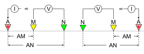
Fig. 447 (Left) Pole-dipole survey configuration with remote source electrode at “infinity. (Right) Dipole-pole survey configuration.

Survey Design

The detectability property of a given survey depends mainly on its ability to inject electrical currents into the mineralization zone. The geologic structures at Mount Isa are primarily steeply dipping geological units striking north-south. This is illustrated in the geologic section and the representative conductivity model.

This alternating sequence of high and low conductivity is an important factor to consider during survey design. To better understand this particular setting, we simulate the flow of current through the expected geology below. The arrow lines show the direction of the currents due to a moving source at the surface. The thin vertical conductors and resistors respectively attract or repel the currents. The best flow into the mineralisation (represented as the circular, conductive body) occurs when the pole is located near 11650, at the eastern edge of the vertical resistive unit (Eastern Quartz Volcanic). The currents are observed to alter their flow paths to penetrate the body. It is also important to note the channeling of currents that occurs because of the conductive Breakaway Shale. Indeed for the dipole-pole case, where the current electrode is beyond the Breakaway Shale (around 12350), the current flows directly into the Breakaway Shale and potentials measured to the west of the shale are small. We will see this problem arise in the next chapter.

Table 11 : DCR simulation over a synthetic Mt. Isa conductivity model without (top) and with (bottom) the conductive mineralized zone. Conductivity values for the different rock units are representative of the geology at Mt Isa.

– + Once Loop Reflect

Conductivity model (color) and current flow (arrows) for a range of source locations (Powered by: SimPEG).

We generate synthetic data for the pole-dipole configuration from the numeric simulation above in order to test the resolving power of our DCR experiment. To assess if this configuration is sensitive to the mineralization at depth, we examine two scenarios; one without, and one with, the deep conductor. These two pole-dipole pseudosections using 15 electrodes spaced 100 meters apart are shown in Fig. 448. The pseudosections look almost identical near the surface but the data differ substantially at lower elevations. To add more insight we invert the two data sets and compare the recovered models.

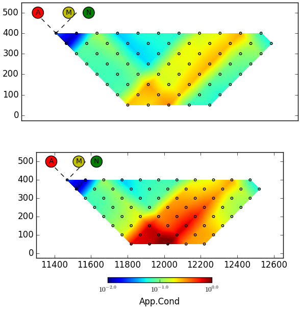
Fig. 448 Pseudo-conductivity section of apparent conductivity for a simulated pole- dipole survey over a geological model without a conductor (top image) and with a conductor (bottom image).

The synthetic data are inverted with a 2D algorithm. A mesh of 20-m by 20-m cells discretized the subsurface. A reference and initial model of 0.05 S/m was used. The recovered models without, and with, the deep conductor are show in Figure Fig. 449. The results show that the deep conductor can be imaged but, because of its close proximity to the conductive shale, and the fact we are using a smooth inversion, it does not appear as a confined conductor. Nevertheless, the results indicate an extended conductor at depth. This is consistent with the images of current density current density that show current being channeled into the body.

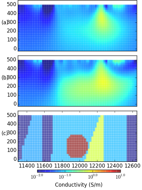
Fig. 449 The recovered 2D conductivity models from the inversion of the pole-dipole data shown in Fig. 448. The middle figure contains the deep conductor and the top lacks a deep conductor. In both figures, the true conductivity model is shown in grey scale for reference.