Interpretation

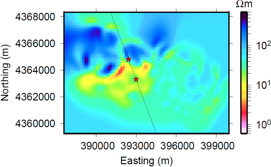
Fig. 402 Depth slice of final inverse model at 1047 m. Two well locations are indicated with red stars. The line connecting the stars indicates where the cross-section in Fig. 404 is taken.

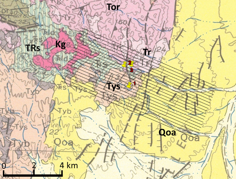
Fig. 403 Cropped geology map ([HJ97]) with the flight lines of the ZTEM survey. The survey consists of 20 lines, separated by 200 m. Each line is approximately 11 km long. Geologic units mapped at the surface are Qoa (surface alluvium), Kg (granites), Tys (non-marine sedimentary rocks), TRs (limestone), Tor (rhyolitic welded tuff), and Tv (volcanic rocks) [Pag65]. The pins show the locations of wells and a DC resistivity survey.

On the previous page, the ZTEM data were processed and inverted. Fig. 402 shows the final recovered model, in UTM coordinates, slices to a depth of 1037 m. The model shows a large conductor as expected, with a large resistive area in the northwest. Resistivities are near the background value in the eastern portion of the model, and this indicates a lack of contrasting lithology within the alluvial fan. The boundary between this unit and the conductive region is indicative of the faults previously mapped along the mountain front, and shown on the geology map. For ease of reference, the geology map is reproduced on this page in Fig. 403.

Several wells were drilled at the survey site in the early 1980s. We specifically looked at two wells logs [TheRCorporation81a, TheRCorporation81b] markes as “1” and “2” in Fig. 403. In well “1”, argillite and siltite comprised the first ~550 m, followed by granite. A mixture of sediments, volcanics, and argillite was found in the first ~250 m in well “2”, followed by granite. Thus, between these two wells, the depth of the granite, considered to be the basement unit, decreases. We expect the granite to be resistive compared to the overlying material. A cross-sectional view (Fig. 404) shows that depth to the granite correlates with the model recovered from the inversion. The depth to the top of the granite basement is marked with black lines underneath the location of the wells. At well “2”, the boundary between the overlying conductor and the underlying resistor agrees with the top of the granite basement. The resistor appears close to t he surface and extends to depth in the western portion of the recovered model and thus likely represents the basement granite. The conductive unit above the granite basement extends deeper at well “1”, indicating a deeper depth to basement. This agrees well with the well data. The difference in depth to basement between the two wells is ~300 m. This difference and the deepening conductor in the 3D model possible relate to faulting. The high conductive zone trends roughly north- west like the mappes faults in the Dixie Valley and its high conductivity may indicate fluid flow or alteration.

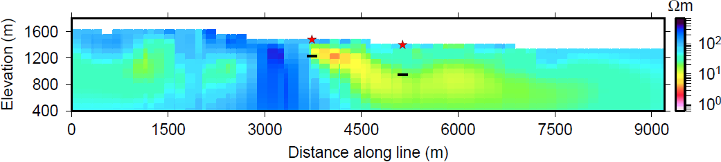
Fig. 404 Cross-section of the model. The cut lies along the lines between wells “1” and “2” in Fig. 402 and looks east. The model is cut-off at the bottom at approximately 1 skindepth. The black lines indicate the depth to granite in the well logs.