Data
Purpose
To define the data of an airborne FDEM system and show the ways of visualizing them.
Definition
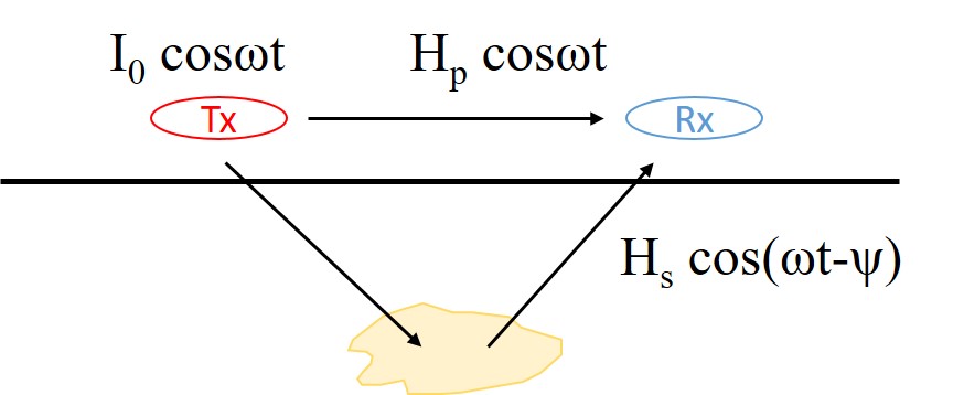
Fig. 186 A time varying current \(I_0 \mathbf{cos}(\omega t)\) generates a primary magnetic field Hpcosωt which induces secondary currents in the subsurface and creates secondary magnetic fields \(H_s \mathbf{cos}(\omega t- \psi )\). Both the primary and secondary fields reach the receiver.
Any time-harmonic signal can be expressed by an amplitude factor times an oscillating term of a sinusoidal function. We denote the transmitter current as \(I_0 \mathbf{cos} \omega t\), which indicates a peak current \(I_0\) and a fixed angular frequency \(\omega\). According to Biot-Savart’s law, the primary magnetic field generated by this current is \(H_p \mathbf{cos} \omega t\), where \(H_p\) can be determined using the distance from the transmitter to any observation point in the whole-space, and the primary field is entirely in-phase with the transmitter current. Then the primary field induces eddy currents in the subsurface. In most cases, this induced current is no longer in-phase with the primary and usually bears a phase lag \(\psi\) (see Circuit Model for EM Induction for the origin and implication of the phase lag). So the secondary magnetic field due to the induction has the form \(H_s \mathbf{cos}(\omega t - \psi)\), where the amplitude \(H_s\) is determined by the distance and geometric coupling. Finally, at the location of receiver, we can observe the primary field \(H_p \mathbf{cos} \omega t\) and the phase-lagged secondary field \(H_s \mathbf{cos}(\omega t - \psi)\).
A FDEM system in practice only measures the secondary field \(H_s \mathbf{cos}(\omega t-\psi)\). The convention in FDEM is to use the primary field \(H_p \mathbf{cos} \omega t\) as the reference to describe the secondary field data. First the secondary field is considered as a linear combination of two orthogonal sinusoidal signals
where \(\mathbf{cos}(\omega t)\) represents a signal in-phase with the source and \(\mathbf{sin}(\omega t)\) represents a signal out of phase with the source. The first term is also called “real”’ and the second term “imaginary” or “quadrature”. Next, the amplitudes of the two sinusoidal signals are normalized by the amplitude of the primary field at the receiver to obtain the data in real and imaginary components
Note the normalization provides significant convenience, as it eliminates the need of timing the measured signals and the effect of the transmitter and receiver’s dipole moments. Because the data are relative quantities, they are denoted as \(H_s/H_p\) and expressed in percent or most often in parts per million (ppm).
Visualizing data
We create a synthetic airborne FDEM data set and illustrate how the acquired data are visualized in practice. The synthetic earth model is a 1 S/m conductive sphere of a 30 m radius buried 20 m deep in a \(10^{-6}\) S/m uniform half-space. Airborne FDEM soundings are measured along 11 survey lines covering a 300 x 300 m area centered at the sphere. The line spacing and in-line sounding spacing are both 30 m. At each sounding, the FDEM system measures the in-phase and quadrature components of Hs/Hp data using horizontal co-planar coils 20 m above the surface in a frequency band from 1 to 100 kHz. The synthetic data are generated by a 3D frequency-domain EM modeling code that approximates the sphere by small voxels.
Map
An airborne FDEM data map is produced by contouring data at a particular frequency as a function of the horizontal location. Click the buttons in the animation below to go through a sequence of maps at different frequencies for both the in-phase and quadrature components. The maps are useful in identifying the horizontal location of the sphere. Realistic data are more complicated than the single peak anomaly in this example, but a map is still a good method for general assessment. The variation of the responses at different frequencies shows that the data at higher frequencies are more sensitive to near surface.
Profile and sounding
An airborne FDEM profile is produced by plotting the data of the same frequency from all the soundings along a flight line. In-phase and quadrature are plotted separately. Fig. 187 (a) shows one profile directly over the sphere. A profile plot can be used to locate the object along the line. Analysis of the profile curves is sometimes used to infer the geometry and orientation of the object. The data can also be plotted as a function of frequency at individual soundings. The sounding plot is particularly useful in indicating whether the system is in resistive limit or inductive limit.
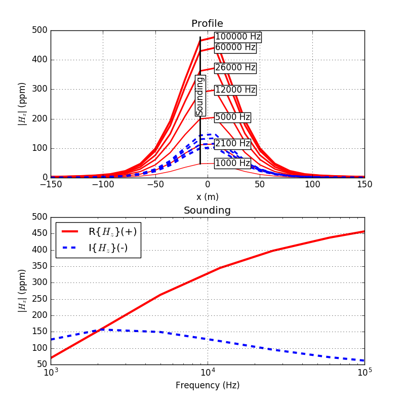
Fig. 187 Top: An airborne FDEM profile over the conductive sphere for a range of frequencies. Bottom: The frequency sounding from a single location marked in the top panel.
Why visualizing
Understanding the underlying physics - Do the real and imaginary components present the general pattern we expect in the 3-loop model? - Does the system operate in a more conductive or more resistive environment? - Are the signs in the data compatible and consistent with the convention that the interpreter uses?
Data quality control - Can we see any suspicious data or outliers? Is there interference from cultural noise? - What is the approximate noise floor in the data?
Qualitative interpretation - Does the relative highs and lows in the data match the general geology or other a priori information we know? - Is there any indication of the sought target in the data? - What is the likelihood of making an informed decision?
Towards an inversion - What is the resolution of the data? - What physical model is appropriate for this data set? - Does the predicted data from the inversion model acceptably match the observed field data? - Is there any important feature in the observed data that is not duplicated by the inversion?