Physics

Purpose

Demonstrate the fundamental physical principles governing the airborne FDEM experiment.

Most of the physics related to airborne FDEM is available in Maxwell I: Fundamentals and Maxwell III: FDEM. Because an airborne FDEM system uses small coils as the transmitter and receiver, geophysicists have developed some representative physical models. Readers are supposed to be familiar with the following concepts.

  • A circuit model for EM induction

  • Sphere excited by a magnetic dipole

  • Magnetic dipole in a whole space

  • Magnetic dipole above a half space

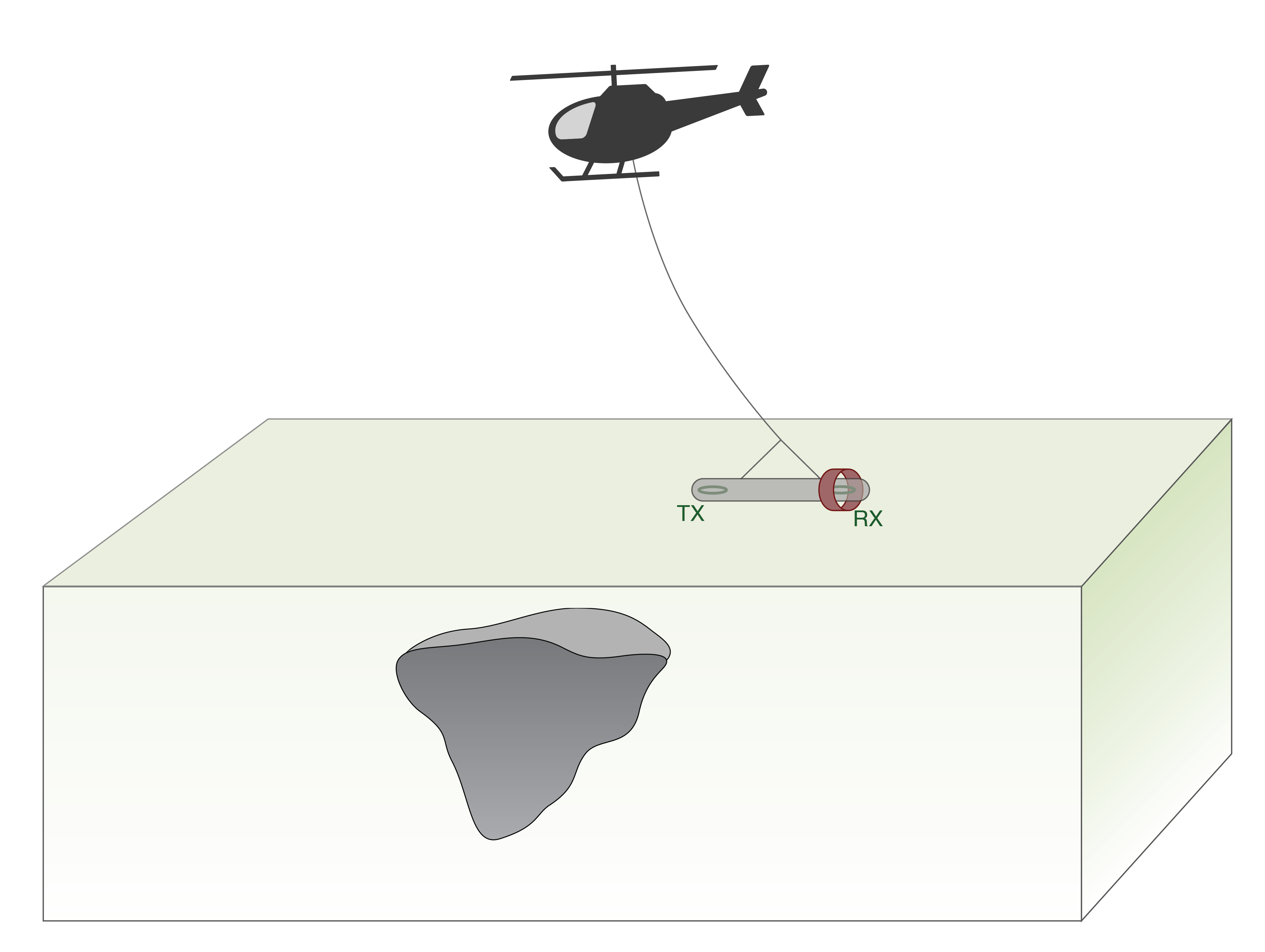
The basic physics of airborne FDEM is illustrated by the animation below. Click through the radio buttons to see how an airborne FDEM system senses a buried conductive object.

Airborne FDEM
airbornefdem

Airborne FDEM survey.
The transmitter and receiver are in the bird towed by the helicopter.
The transmitter produces a time-varying primary magnetic flux.
The time-varying magnetic fields produce electric fields everywhere and thus induce currents in the conductive target according to Lenz' law.
The induced currents produce a secondary magnetic field.


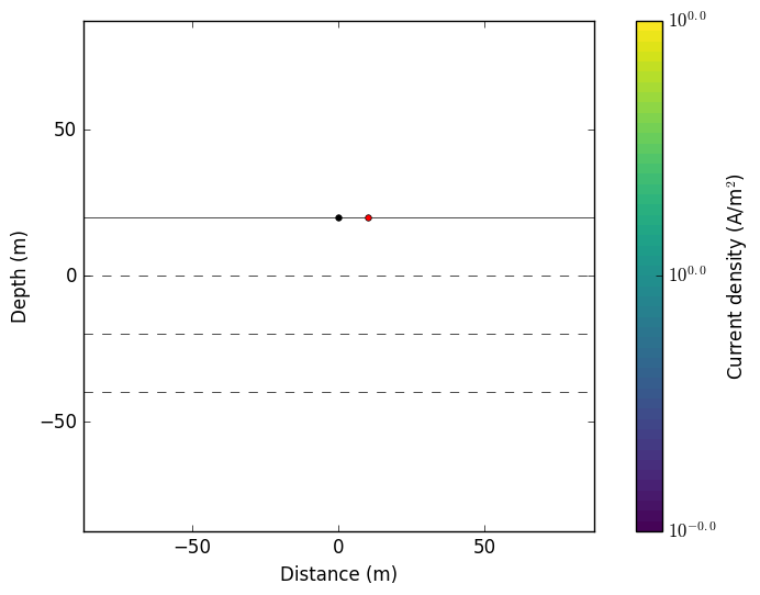
Two typical earth models are of particular interest in airborne EM: the 1D layered earth model and the sphere-in-halfspace model. Here we illustrate the basic physics involved in airborne FDEM with a small horizontal loop source (a vertical magnetic dipole) over a three-layer earth model. The receiver is another horizontal loop coil measuring the magnetic field. Both loops are at the same altitude 20 metres above the surface and are separated by 10 metres. Click through the radio buttons to explore the problem.

Airborne FDEM
airbornefdem_demo

Airborne FDEM survey over a layered 1D Earth.
The 1D conductivity earth model. Top layer: 0.1 S/m and 20 m thick; Second layer: 1 S/m and 20 m thick; Basement: 0.1 S/m. The source and receiver are marked by the black and red dots respectively.
The harmonic vertical magnetic dipole source (black dot) at 100 Hz induces electrical current (showing amplitude) below the surface. Note the geometric fall-off of the current intensity from the source location to large depths/distances, and the enhanced current in the conductive layer.
The harmonic vertical magnetic dipole source (black dot) at 10 kHz induces electrical current (showing amplitude) below the surface. Note the stronger concentration of current near the surface, if compared to the 100 Hz source.
The secondary magnetic field (showing the real component) everywhere in the whole-space generated by the induced current in the earth.
The receiver (red dot) measures the secondary magnetic field at multiple frequencies.