Purpose

Here, we present a workflow for UXO classification. We then discuss methods for removing geological responses.

Interpretation

In many cases, the number of clutter items far exceeds the number of ordnance items within the survey area. As a result, data processing and interpretation techniques are used to differentiate ordnance items from clutter and produce a prioritized dig list of targets for excavation. A workflow showing the processing steps for UXO classification is shown in Fig. 272.

Workflow for UXO Classification

Fig. 272 Workflow for UXO classification.

Digital Geophysical Map (DGM): These are visually represented data collected during the UXO survey.

Target Picking: In this step, we identify anomalies down to a pre-defined amplitude threshold for further processing. The threshold is usually set based upon the minimum expected data amplitude for the smallest target of interest (i.e. UXO) at a site.

Cued Interrogation: Here, high-quality data are collected over each picked target. Despite adding time and expense, this step frequently provides the level of data quality required to accurately classify each picked target.

Feature Estimation: Each anomaly from cued interrogation data is characterized by estimating features. This allows us to discern UXOs from non-hazardous clutter. Features may be directly related to the observed data (e.g. anomaly amplitude at the first time channel), or they may be the parameters of a physical model.

The former approach is appealing in its simplicity but is generally not an effective strategy. For example, an ordnance item at depth will produce a small anomaly amplitude and might be left in the ground when using a dig list based solely upon anomaly amplitude. Most classification strategies therefore use physical modeling to resolve such ambiguities.

Detailed descriptions of the physical modeling used for processing electromagnetic data are given in Bell et al. ([BBT01]), Pasion and Oldenburg ([PO01]) and Zhang et al. ([ZCY+03]); note that models were presented in physics. In the feature estimation stage, these models are fit to the observed EM data for each target anomaly (Fig. 273). The model is parameterized by target location (\(x,y,z\)), orientation (\(\theta,\phi\)) and polarizabilities (\(L_{x'}, L_{y'}, L_{z'}\)). The polarizabilities are intrinsic to each target and can therefore be used to make classification decisions.

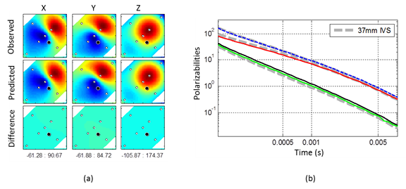
Fig. 273 Fitting Metal Mapper data using the parameterized model. (a) Observed data (top row) and data predicted by fitting a physical model to the observed data (middle row). Bottom row shows a negligible difference between observed and predicted data, indicating a good fit. (b) Estimated polarizabilities (colored lines) recovered via fitting, overlain on known polarizabilities for 37 mm projectiles. The excellent correspondence between recovered and reference polarizabilities indicates – with high confidence – that the detected target is a 37 mm item.

Quality Control: Once the data has been fit using a parameterized model, it is important to assess how well the model is able to explain the data. This can be done by examining the difference between the observed data and data predicted using the parameterized model.

Classification: Here, the polarizations recovered for each target are compared against those within a library of known ordnance items. UXO classification is successful when the recovered polarizations match those of a known ordnance item. As expected, the polarizations of clutter objects will not match any of the polarizations contained within the library.

In Fig. 274 we compare typical polarizabilities for UXO and non-UXO items. The primary polarizability (\(L_1\)) aligns with the long axis of the target. UXOs generally have larger amplitudes and slower decaying polarizabilities relative to small clutter. Shape information is encoded in the secondary polarizabilities (\(L_2\) and \(L_3\)). Most UXOs have a circular cross-section and will have \(L_2 \approx L_3\). In contrast, for irregularly-shaped clutter these parameters are significantly different. These differences in the polarizabilities allow us to distinguish between buried UXOs and clutter.

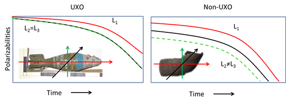
Fig. 274 Comparison of representative polarizabilities for UXO and non-UXO items.

Geological Noise

Generally the EM responses from UXOs are significantly stronger than the EM responses from the host medium. In these cases, it is acceptable to neglect the response from the host medium. However, there are certain geological environments in which this assumption is invalid. As an approximation, it is common to neglect coupling and consider the UXO and geological responses as separable, thus:

\[B_{tot} = B_{s} + B_{geo}\]

It is important to recognize when the geological response is significant. If treated properly, the geological response can be removed from the observe data, thus isolating the target’s response.

Conductive Backgrounds

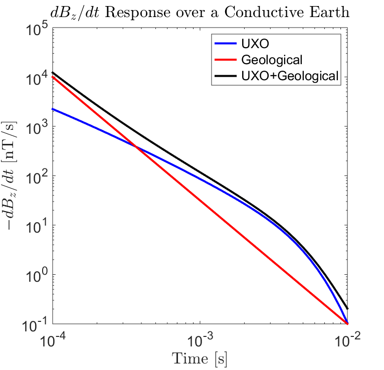
Fig. 275 Example of the Earth’s inductive response masking the early time response from a UXO.

In regions where the local geology is very conductive (\(\sigma > 0.1\) S/m), the Earth’s inductive response becomes significant. The transient response from a conductive Earth is generally recognized as having a \(B_z(t)\) response which decays as \(t^{-3/2}\) and a \(dB_z/dt\) response which decays as \(t^{-5/2}\). Generally speaking, the Earth’s inductive response decays much faster than the responses exhibited by UXOs. As a result, inductive responses from the Earth are more likely to impact UXO data at earlier times.

Processing steps are sometimes added in order to remove the Earth’s inductive response. A common approach is to fit the background response using the best-fitting local half-space model. Data are then forward modeled over the target and subtracted from the observed data.

Magnetic Backgrounds

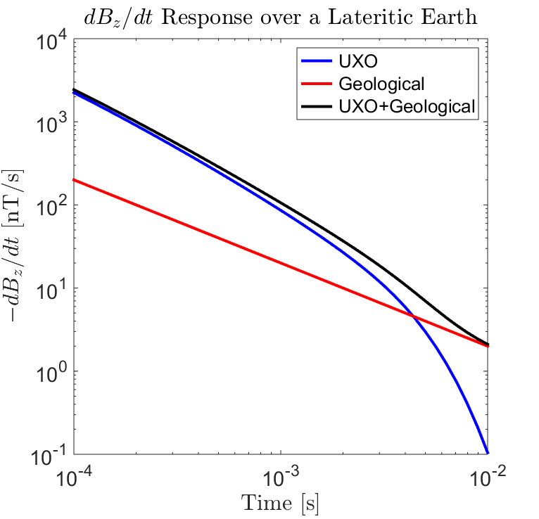
Fig. 276 Example of the VRM response masking the late time response from a UXO.

TEM methods become less effective in regions where lateritic topsoils are prominent. Lateritic soils are highly weathered, rich in iron-oxide minerals and found within tropical and sub-tropical climates. Lateritic soils are known to exhibit strong viscous remanent magnetization (VRM) (link). As a result, these soils exhibit a transient magnetic response which has been shown to mask the TEM anomalies exhibited by UXOs. The VRM response is characterized as having a \(B(t)\) response which decays proportional to \(ln(t)\). Meanwhile, the \(dB/dt\) response decays proportional to \(t^{-1}\). VRM responses commonly mask the late time responses exhibited by UXOs. However because VRM and UXO responses decay similarly over early and mid-times, they can be hard to differentiate.

Processing steps are sometimes added in order to remove the Earth’s VRM response. A common approach ([Pas07]) is to fit the background response using the best-fitting local half-space model. Data are then forward modeled over the target and subtracted from the observed data. 3D modeling approaches are currently being developed ([Cow16]).