Purpose
Here, the fundamentals of GPR survey design are discussed.
Survey Design
In order to design an effective GPR survey, it is important to ask the following questions:
What survey configuration would be best for resolving the target?
What is the optimum position and orientation for the transmitter and receiver antennas?
How deep into the Earth do I need to image?
What are the smallest features I need to image? What resolution is required?
What operating frequency should be used?
What are the physical properties of the Earth and how do they impact my survey?
How should I orient my survey profile relative to a geophysical target?
What is the ideal station spacing and transmitter-receiver separation?
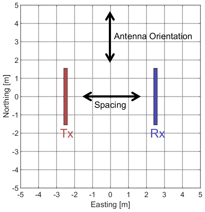
Fig. 242 GPR orientation.
Optimum Antenna Position
For a successful GPR survey, the transmitter and receiver antennas must be positionned so that signals emitted by the transmitted are most effectively measured by the receiver. This is generally accomplished by orienting the transmitter and receiver antennas parallel to one another, and positioning the receiver antenna at a location perpendicular to the orientation of the transmitter antenna (Fig. 242). The details of this are discussed below.
Signal Intensity and Location
Fig. 243 Radiation pattern showing the electric field for a half-width electric dipole (Source ).
The intensity of the radiowave signal generated by the transmitter antenna is not the same in all directions. In fact, the intensity of the signal in one direction relative to the transmitter antenna may be much weaker compared to the intensity in another direction. Ultimately receiver antennas are positioned to record signals along the direction of highest intensity.
The radiation pattern for a particular transmitter antenna depends on its shape and operating frequency. In general, the intensity of the EM radiation emitted by a dipole antenna is strongest in directions perpendicular to the orientation of the antenna. For a half-width dipole antenna, this is shown in Fig. 243. As we can see, it would be ill-advisable to place the receiver antenna in-line with the transmitter antenna in this case.
Orientation and Coupling
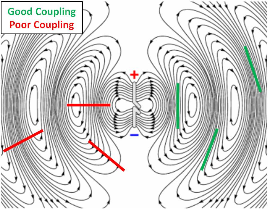
Fig. 244 Ideal and poor receiver antenna orientations for a half-width dipole transmitter (Adapted from source image ).
Radiowave signals emitted by the transmitter antenna are polarized, meaning they carry electric fields which oscillate in particular directions. Because of this, the receiver antenna must be oriented in a direction such that it sensitive to the incoming signal. Receiver antennas measure GPR signals most effectively when they are oriented along the direction of the electric field. In this case, the transmitter and receiver are well-coupled. Examples of good coupling and poor coupling for a half-width dipole antenna are shown in Fig. 244. As we can see, many of the ideal receiver orientations are parallel to the transmitter antenna.
Probing Distance
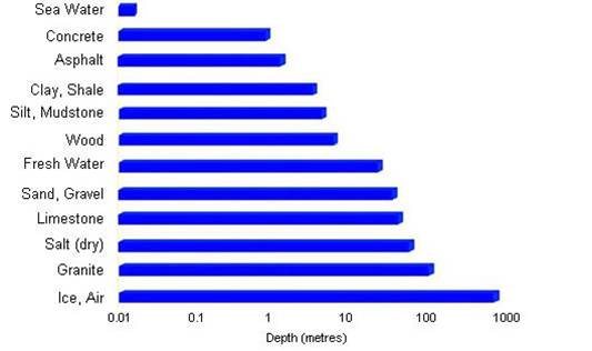
Fig. 245 Proving distances for GPR signals for various materials.
Probing distance characterizes the maximum depth in which GPR signals can be used to obtain information about subsurface structures. In some cases it is referred to as depth of penetration. For materials which have larger skin depths, radiowaves can penetrate deeper into the ground and still provide a sufficiently strong returning signal.
As a general rule, the probing distance (\(D\)) is approximated 3 skin depths. If we assume the Earth is non-magnetic (\(\mu_r = 1\)):
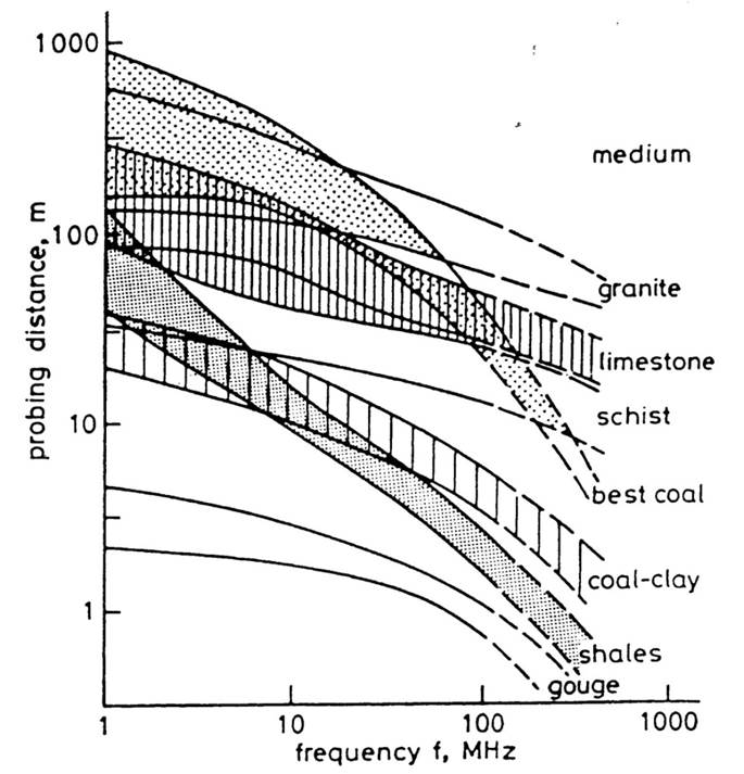
Fig. 246 Probing distance for various materials from 1 MHz through 1 GHz.
On the right we see figures which show probing distances for various materials. Using these figures, we can see that:
In general, as the frequency increases, the skin depth decreases and the probing distance decreases.
Frequencies used for GPR are \(\sim\) 1 GHz. Therefore, the probing distances for GPR signals are generally quite shallow.
It is very difficult for GPR signals to penetrate concrete and asphalt, as the probing distance is only about 1 m for GPR.
Water saturated sedimentary rocks, such as clays and sandstones, have much lower probing distances than dry sedimentary rocks.
Rocks saturated with sea water have much smaller probing distances than rocks saturated with fresh water.
The probing distances for hard rocks (granites, limestones, schists…) is quite large.
Resolution
The choice in operating frequency is a very important aspect of GPR survey design. When designing a survey, we must ensure that GPR signals can penetrate to sufficient depth in order to image the target. However, we must also ensure that frequencies contained within the GPR signal provide sufficient resolution. We will show that although higher operating frequencies can be used to obtain higher resolution images of the subsurface, higher frequency GPR signals cannot penetrate very deeply.
Vertical Resolution for Layers
In order for a layer to be detected using a GPR survey, it must be sufficiently thick compared to the wavelength of the incoming wavelet. As a general rule, the layer must be at least 1/4 the wavelength of the incoming wavelet to be detectable. Thus:
where \(L\) is the layer thickness, \(c/\!\sqrt{\varepsilon_r}\) is the propagation velocity for radiowaves, \(\Delta t\) is the pulse width and \(f_c\) is the central frequency. As we can see from this expression, higher frequencies/shorter pulse widths are required to observe smaller features. This means higher frequencies/shorter pulse widths are used for higher resolution surveys.
Horizontal Resolution for Objects
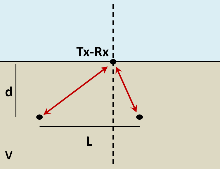
When the resolution of the survey is sufficient, returning signals from separate buried objects are distinguishable. However, if buried objects are too close to one another, their respective returning GPR signals can be hard to differentiate. In general, we can distinguish the signals from two nearby objects so long as:
where \(V\) is the propagation velocity, \(f_c\) is the central frequency for the wavelet, \(d\) is the depth to the objects and \(L\) is the horizontal separation distance of both objects. We can see from this equation, that by reducing the pulse length, we can image objects that are closer together. Additionally, it is harder to distinguish objects which are further away from the transmitters and receivers.
Common Offset Considerations
Transmitter-Receiver Separation
If a zero-offset configuration is being used, this aspect of survey design is redundant. For a common offset survey however, the transmitter-receiver separation is very important. Surveys are successful when both the transmitter and receiver antennas are sensitive to the target region. For each antenna, this region is defined by the refraction focusing peak and depends on the critical refraction angle of the air-Earth interface. For several relative permittivities, this is shown in Fig. 247. From this, an estimate of the optimum antenna separation (\(S\)) is given by:
where \(K\) is defined here as the Earth’s relative permittivity and \(d\) is the approximate depth of the target. If little is known regarding the survey area, then the rule-of-thumb is to set \(S \approx d/5\). It should be noted however, that depth resolution can be increased by decreasing the antenna separation.
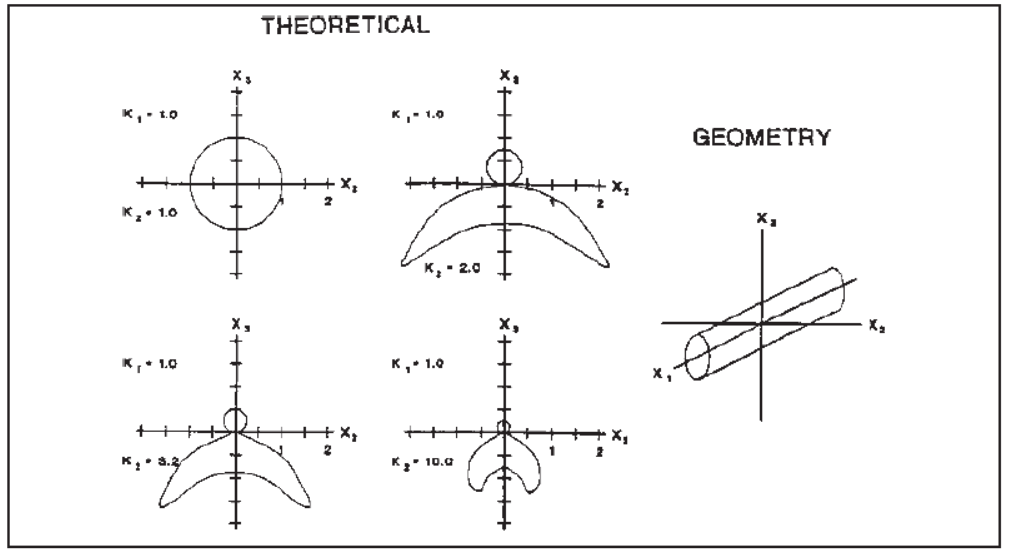
Fig. 247 Variations in antenna radiation patterns resulting from various relative permittivities (\(K\)) for the Earth. The orientation of the antenna is depicted on the right.
Station Spacing
When selecting a station spacing, we want to avoid spatial aliasing. This is accomplished by using a station spacing which does not exceed the Nyquist sampling interval. The Nyquist sampling interval is one quarter the wavelength of the signal as it propagates through the medium. Thus we should use a station spacing (\(\Delta x\)) defined by:
where \(\lambda\) is the signals wavelength, \(f_c\) is the central operating frequency of the transmitter, \(c = 3 \times 10^8\) m/s is the speed of light and \(\varepsilon_r\) is the relative permittivity of the medium. When the station spacing is too large, the data will become unable to adequately define structures such as steeply dipping layers. Although adequate spatial sampling is important, there are no significant benefits from over-sampling.
CMP and WARR Considerations
Transmitter-Receiver Separation
For common midpoint (CMP) and wide angle refraction reflections (WARR) surveys, the minimum transmitter-receiver separation should not exceed the Nyquist sampling interval (\(\Delta x\)) defined above. For each successive reading, the transmitter-receiver separation should increase by \(\Delta x\); for CMP surveys, the transmitter and receiver are moved a distance \(\Delta x/2\) after each reading. The maximum separation distance for both CMP and WARR surveys generally does not exceed 1-2 times the depth of the target interface.
Profile Orientation and Spacing
In general, survey lines run perpendicular to the trend of subsurface features we want to investigate. For example, if we are trying to locate a buried pipe which is oriented North-South, we would use GPR to images along an East-West profile. For a dipping layer, we would want to profile perpendicular to the strike direction of the interface. A major reason for choosing this orientation is that for discrete objects, it will result in hyperbolic radargram signatures which can be easily interpreted. In addition, more information can be gathered using fewer survey lines.
Survey line spacing depends on the extent of variation in subsurface features along the trend direction (pipe orientation or strike direction). If there is little to no variation, only one profile line may be needed to accurately characterize the target features. If there are significant variations, the profile line spacing should be set according to the Nyquist sampling interval.