Interpretation
Purpose
To show how airborne TDEM data are processed and inverted to reveal meaningful information about the earth structure.
Interpretation is the process that extracts information in the delivered data to make decisions or to derive geologic knowledge. Depending on the specific geologic questions asked, and the resources available, geophysicists can choose from a wide spectrum of approaches ranging from trivial and low- resolution to sophisticated and high-resolution.
Preliminary interpretation
Data plotting
Significant amount of information, especially the relative distribution of conductivity, can be obtained by just plotting the data. Sometimes simple data transform techniques can also be used to isolate the anomaly and aid the interpretation. This type of approach can include: direct data plotting, data- conductivity transform, empirical template method, etc. Those simple methods were once the mainstream, but have shown drawbacks in complex geological setting and lack the ability to decode the conductivity values from the data. However, it still has its value in data quality control and preliminary interpretation.
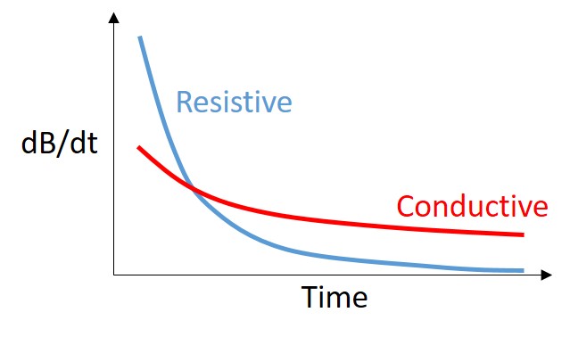
Fig. 197 A conductive terrain has a slowly-decaying dB/dt response. For most time (except very early time), a high value in dB/dt indicates the existance of conductive objects.
For a time domain system, the voltage measured off time at the receiver is roughly an exponentially decaying function of time. The decay rate is an indicator of the overall conductivity of the ground: good conductors have slower decays (greater time constant) and poor conductors have faster decays (smaller time constant).
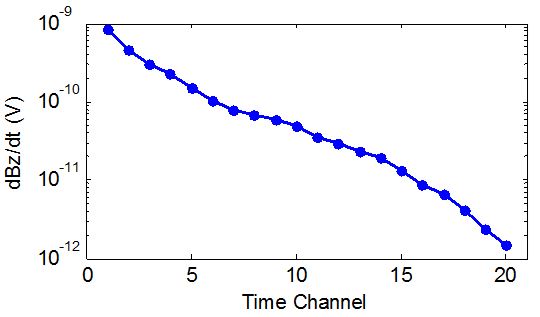
Fig. 198 Example sounding showing variation of conductivity at depth. A slowly-decaying dB/dt from time channel 7 to 15 indicates a more conductive layer underneath.
Time constant method offers a first-order interpretation of the overall conductivity of the ground. For example, we can infer the overall conductivity by examining how fast the dB/dt response decays in time. Using delay time (time channel) as a proxy of depth, we can qualitatively estimate the variation of conductivity as a function of depth.
Apparent conductivity
Apparent conductivity is another semi-qualitative method that further ties the data to the conductivity of the ground. It is defined as the conductivity of a uniform half-space that would generate the same data at a particular time channel. It can be considered as a lumping averaging of the conductivities around the measurement location. Despite its blending effect, it provides qualitative insight about how the conductivity varies from shallow (early times) to deep (late times). Using the concept of diffusion distance, apparent conductivities calculated at time channels can be assigned a pseudo- depth, so a depth image can be generated for a preliminary interpretation. This technique is usually referred to as conductivity-depth imaging/transform (CDI/CDT).
Quantitative Inversion
1D layered earth inversion
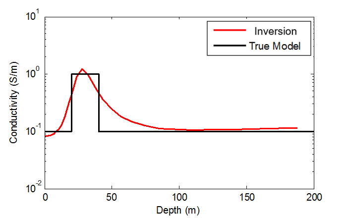
Fig. 199 1D layered earth inversion of the 3-layer model.
This approach assume the earth’s conductivity only varies as a function of depth. At each measurement location, the inversion find a layered model that explains the entire decay curve in time. Fig. 199 shows the 1D inversion result of the 3-layer example in Physics. Many layered models at multiple locations then can be stitched together to form a pseudo-3D volume for visualization. The conductive layer from 20 to 40 m depth is reasonably recovered by the inversion, although the interfaces are not sharp becasue of the smooth constraint used in the inversion.
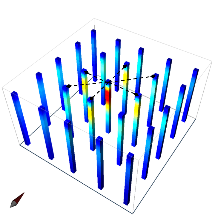
Fig. 200 1D layered earth inversions of the sphere model.
For the data from the sphere model, 1D inversion can still be performed at individual stations to provide information about local changes in conductivity. Fig. 200 presents such 1-D models in a 3-D space for the sphere example, but the lack of lateral continuity makes it difficult to interpret. Many layered models at multiple locations then can be stitched together to form a pseudo-3D volume for model visualization. Advanced techniques can also consider the correlation between adjacent locations by imposing lateral constraints.
Here we use the synthetic data set generated for the sphere model as an example to demonstrate the 1D inversion technique. The earth is horizontally divided into 20 layers from the surface to the basement. The top layer is 0.5 m thick, and the layers are gradually thickened at a rate of 1.2 toward the depth. The dBz/dt data are noise-free, but we assume that there is a 5% noise in all time channels. The animation below compares the observed (top) and predicted (bottom) data and the pseudo-3D conductivity model obtained by stitching the individual 1D layered models. The sphere is reasonably imaged on the cross section. Although the sphere’s geometry is distorted and its conductivity value is underestimated, the inversion still reasonably reflects the correct horizontal location and the depth to the sphere’s top.
2D/3D inversion
The previous interpreting methods all assume the earth has a particular structure so simplified calculations can be used. Any violation of those assumptions would result in failures. A 3D inversion discretizes the entire earth to many discrete cells, each of which has a constant conductivity. Then the Maxwell’s equations are solved on the mesh. The obtained images of the subsurface are in 3D voxel format. 3D inversions provides the best resolution and works for any complicated models, but it is more computational expensive. A 2D inversion is similar to a 3D inversion, except that the physical property along the strike direction is constant, so there are fewer variables in the model.