Data

ZTEM data consists of the vertical magnetic field \(\mathbf{H}_z\) collected along survey lines with an airborne system. The horizontal magnetic fields \(\mathbf{H}_x\) and \(\mathbf{H}_y\) are measured at a referecen station on the ground. Generally, the reference station is placed in a location where the earth structure is 1D.

Similar to the measured MT data, the ZTEM system records a time-series of the magnetic field. The data are then binned and processed to generate transfer functions in the frequency domain [HO10b]. For more information about converting the time-series into frequency domain, see the MT data page.

Similar to MT which uses the impedance, ZTEM data or tipper data are transfer functions. For this method, the transfer functions are calculated from relating the vertical magnetic field at locations \(\mathbf{r}\) and the horizontal magnetic fields at the base station located at \(\mathbf{r}_0\). :

(496)\[\mathbf{H}_z (\mathbf{r}) = T_{zx}(\mathbf{r},\mathbf{r}_0) \mathbf{H}_x (\mathbf{r}_0) + T_{zy}(\mathbf{r},\mathbf{r}_0) \mathbf{H}_y (\mathbf{r}_0)\]

By taking the ratios of the vertical and horizontal fields, the influence of the unknown source field is removed (similar to the MT method).

In order to solve Equation (496), two independent polarizations are required:

\[\mathbf{H}_{z1} (\mathbf{r}) = T_{zx} \mathbf{H}_{x1} + T_{zy} \mathbf{H}_{y1}\]

\[\mathbf{H}_{z2} (\mathbf{r}) = T_{zx} \mathbf{H}_{x2} + T_{zy} \mathbf{H}_{y2}\]

The transfer functions are then solved for as following:

\[T_{zx} = \frac{\mathbf{H}_{y2} \mathbf{H}_{z1} - \mathbf{H}_{y1} \mathbf{H}_{z2}}{\mathbf{H}_{x1}\mathbf{H}_{y2} - \mathbf{H}_{x2}\mathbf{H}_{y1}}\]

\[T_{zy} = \frac{-\mathbf{H}_{x2} \mathbf{H}_{z1} + \mathbf{H}_{x1} \mathbf{H}_{z2}}{\mathbf{H}_{x1}\mathbf{H}_{y2} - \mathbf{H}_{x2}\mathbf{H}_{y1}}\]

The transfer functions are complex and thus have both a real and an imaginary component.

Consider the example below where a conductive block is buried in a uniform halfspace. The tipper data are forward modelled and the real and imaginary components of \(T_{zx}\) and \(T_{zy}\) are shown in Figure Fig. 211. In each case, the data contain a high and low peak over the conductive block and the orientation of the anomaly depends on which transfer function is plotted.

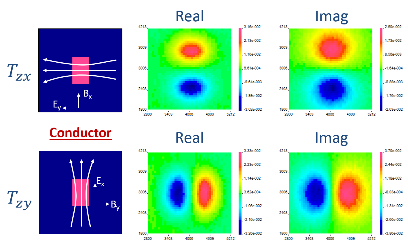
Fig. 211 Real and imaginary components of tipper data for a conductive block in a halfspace.

For a halfspace or uniformly layered earth, the tippers are zero, meaning that no information is available. Therefore, ZTEM data are only sensitive to 3D structures.