Point current source and a conducting sphere

In this section, we build up an analytical solution for a conducting sphere in the presence of a point current source. This is accomplished in two steps:

1. A solution for the electric scalar potential, due to a point current source within a wholespace of resistivity \(\rho\), is solved. This solution is then re-expressed within a polar coordinate system and decomposed into a sum of spherical harmonic modes.

2. The solution for a conducting sphere within a wholespace is then determined by solving a boundary value problem for each spherical harmonic.

This solution is built upon in Effects of Topography to investigate the effects of of a hemispherical depression at the Earth’s surface on the behaviour of currents and potentials in a direct current resistivity experiment.

Electric Potential from a Current Source within a Wholespace

Let us consider the case where an electrical current \(I\) is being injected into a wholespace with resistivity \(\rho\), at location (\(x,y,z\)) = (\(x_0,0,0\)). Assuming the medium is lossless, this results in a current density \(J\) which flows radially outwards from the source, with magnitude:

\[J = \frac{I}{4 \pi R^2}\]

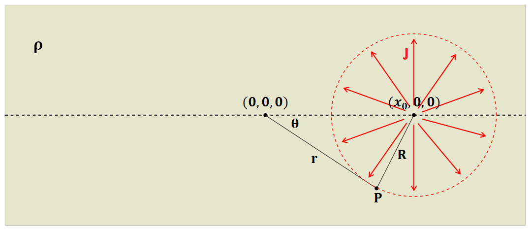
Fig. 80 Diagram showing the setup for computing the potential due to a wholespace.

where \(R\) is the distance from the source to a point of measure \(P\), and \(4\pi R^2\) is the area of a ball centered at the source. Because our problem is electrostatic, \(\vec E = - \nabla \phi\) according to Faraday’s law. The scalar electric potential \(\phi\) can be obtained by integrating the electric field from \(R\) to \(\infty\). By substituting Ohm’s law (\(\vec E = \rho \vec J\)) into the path integral:

\[\phi = - \int_R^\infty \vec E \cdot d\vec l = - \int_R^\infty \frac{\rho I}{4 \pi r^2} dr = \frac{\rho I}{4\pi R}\]

For reasons which will becomes apparent in the next section, we would like to re-express \(\phi\) in terms of a radial coordinate system (\(r,\theta,\phi\)), centered at (\(x,y,z\)) = (0,0,0). Because the points which represent the problem geometry do not necessarily form a right-triangle, \(R\) must be expressed using the cosine law:

\[R = \sqrt{x_0^2 + r^2 - 2rx_0 cos \theta \;}\]

For solutions where \(r<x_0\), \(1/R\) can be split into a sum of spherical harmonic modes using the binomial theorem:

(354)\[\begin{split}\frac{1}{R} &= \frac{1}{x_0} \Bigg [ 1 + \Bigg ( \frac{r}{x_0} \Bigg )^2 - 2 \frac{r}{x_0} cos \theta \Bigg ]^{-1/2} \\ &= \frac{1}{x_0} \Bigg [ 1 + \frac{r}{x_0}cos \theta + \Bigg ( \frac{r}{x_0} \Bigg )^2 \Bigg ( \frac{3}{2} cos^2 \theta - \frac{1}{2} \Bigg ) + \; \dotsb \; \Bigg ] \\ &= \frac{1}{x_0} \sum_{n=0}^\infty \Bigg ( \frac{r}{x_0} \Bigg )^n P_n \big (cos \theta \big)\end{split}\]

where \(P_n \big (cos \theta \big )\) is the Legendre polynomial of order \(n\). Because Legendre polynomials have magnitudes less than unity for \(n>0\), and \(r<x_0\), the infinite series in Eq. (354) is bounded and converges as \(n \rightarrow \infty\). A similar approach for \(r > x_0\) can be expressed as follows:

(355)\[\begin{split}\frac{1}{R} &= \frac{1}{r} \Bigg [ 1 + \Bigg ( \frac{x_0}{r} \Bigg )^2 - 2 \frac{x_0}{r} cos \theta \Bigg ]^{-1/2} \\ &= \frac{1}{r} \Bigg [ 1 + \frac{x_0}{r}cos \theta + \Bigg ( \frac{x_0}{r} \Bigg )^2 \Bigg ( \frac{3}{2} cos^2 \theta - \frac{1}{2} \Bigg ) + \; \dotsb \; \Bigg ] \\ &= \frac{1}{r} \sum_{n=0}^\infty \Bigg ( \frac{x_0}{r} \Bigg )^n P_n \big ( cos \theta \big )\end{split}\]

Similar to Eq. (354), since \(x_0<r\), the infinite series in Eq. (355) is also boundary and conveges as \(n\rightarrow\infty\). Therefore using Eqs. (354) and (355), the electric scalar potential \(\phi\) can be expressed as an infinite sum of spherical harmonic modes, where:

(356)\[\phi = \frac{I\rho}{4 \pi} \sum_{n=0}^\infty \frac{r^n \, P_n \big (cos \theta \big )}{x_0^{n+1}} \; \; \; \textrm{for} \; \; \; r<x_0\]

and

(357)\[\phi = \frac{I\rho}{4 \pi} \sum_{n=0}^\infty \frac{x_0^n \, P_n \big (cos \theta \big )}{r^{n+1}} \; \; \; \textrm{for} \; \; \; x_0<r\]

Unfortunately, this method cannot be used to find a bounded and convergent series for \(r=x_0\).

Electric Potential for a Conducting Sphere in a Wholespace

Let us now consider the electrical scalar potential at \(P\) in the presence of a conducting sphere of radius \(a\) and resistivity \(\rho_1\), centered at the origin. Once again, a current of \(I\) is injected at (\(x_0,0,0\)). Due to the radial symmetry of the problem, \(\partial /\partial \phi = 0\). Away from the source, the electric field is divergence free. As a result, \(\phi\) can be expressed in terms of the following 2d Poisson’s equation:

(358)\[\nabla^2 \phi = \frac{1}{r} \frac{\partial }{\partial r} \big ( r^2 \big ) \frac{\partial \phi}{\partial r} + \frac{1}{r^2 sin \theta} \frac{\partial}{\partial \theta} \Bigg ( sin \theta \frac{\partial \phi}{\partial \theta} \Bigg ) = 0\]

The boundary conditions for our problem state that \(\phi\), and current flow normal to the sphere’s surface, are continuous at \(r=a\). Therefore:

(359)\[\phi = \phi_1 \; \; \; \textrm{and} \; \; \; \frac{1}{\rho} \frac{\partial \phi}{\partial r} = \frac{1}{\rho_1} \frac{\partial \phi_1}{\partial r} \; \; \; \textrm{at} \; \; \; r=a\]

For a source which is outside the sphere (\(a < x_0\)), the desired solution for the potential is:

(360)\[\phi = \frac{I \rho}{4\pi R} + \sum_{n=0}^\infty A_n \frac{1}{r^{n+1}} P_n \big ( cos \theta \big ) \; \; \; \textrm{for} \; \; \; r>a\]

and

(361)\[\phi_1 = \sum_{n=0}^\infty B_n r^n P_n \big ( cos \theta \big ) \; \; \; \textrm{for} \; \; \; r<a\]

This makes sense considering \(1/r\) terms within the sphere would be infinite as \(r \rightarrow 0\), and \(r\) terms outside the sphere would be infinite as \(r \rightarrow \infty\). Because Legendre polynomials can be used to form an orthogonal set of basis functions, coefficients \(A_n\) and \(B_n\) may be determined independently for each \(n\). Using locations \(r<x_0\), Eq. (356) can be substituted into Eq. (360). This can be use to solve Eq. (358), using boundary conditions from (359) for each harmonic mode \(n\). The resulting coefficients are given by:

\[A_n = \frac{I \rho}{4\pi} \Bigg ( \frac{a^{2n+1}}{x_0^{n+1}} \Bigg ) \Bigg ( \frac{n \big ( \rho_1 - \rho \big )}{n\rho + \big (n+1 \big )\rho_1} \Bigg )\]

and

\[B_n = \frac{I\rho}{4\pi} \Bigg ( \frac{1}{x_0^{n+1}} \Bigg ) \Bigg ( \frac{\big ( 2n+1 \big )\rho_1}{n\rho + \big ( n+1 \big )\rho_1} \Bigg )\]

Therefore, the electric scalar potential observed outside the sphere is equal to:

(362)\[\phi (r, \theta ,\phi) = \frac{I\rho}{4 \pi} \Bigg [ \frac{1}{R} + \sum_{n=0}^\infty \frac{a^{2n+1}}{\big (x_0 \, r \big )^{n+1}} \Bigg ( \frac{n \big ( \rho_1 - \rho \big )}{n\rho + \big (n+1 \big )\rho_1} \Bigg ) P_n \big ( cos \theta \big ) \Bigg ]\]

Eq. (362) can be split into two terms: the potential for a wholespace from Eq. (357), and an anomalous potential which results from the exstence of a conducting sphere. Python code functions which evaluate above solution is given at DC sphere code.

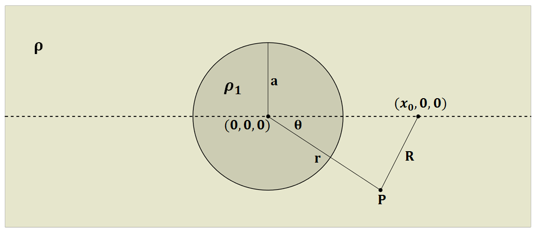
Fig. 81 Diagram showing the setup for computing the potential due to a conductive sphere in a wholespace.

Variables

\(\rho\)	Resistivity of the whole-space
\(\rho_1\)	Resistivity of the sphere
\((0,0,0)\)	Origin of the coordinate and center location of the sphere
\((\pm x_0,0,0)\)	Location of the point current source, which has to be alined with \(x\)-axis
\(x_0\)	Distance from current source from the origin (a postive scalar value)
\(r\)	Distance from the origin to the measurement point \(P(x,y,z)\)
\(R\)	Distance between the measurement point (\(P\)) and the point current source
\(\theta\)	Angle between the measurement point (\(P\)) and the point current source
\(a\)	Radius of the sphere (m)
\(I\)	Intenisty of the current
\(\phi\)	Total potential outside of the sphere (\(r > a\))
\(\phi_1\)	Total potential inside of the sphere (\(r < a\))