Conducting sphere in a uniform electric field

A sphere in a whole-space provides a simple geometry to examine a variety of questions and can provide powerful physical insights into a variety of problems. Here we examine the case of a conducting sphere in a uniform electrostatic field. This scenario gives us a setting to examine aspects of the DC resistivity experiment, including the behavior of electric potentials, electric fields, current density and the build up of charges at interfaces. This work follows the derivation in [WH88] and is supported by apps developed in a binder.

Setup

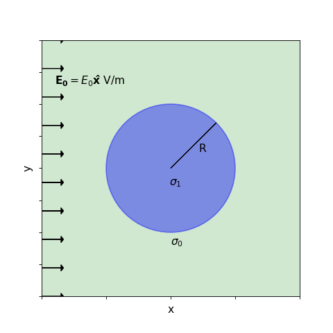
The problem setup is shown in the figure below, where we have

• a uniform electric field oriented in the \(x\)-direction: \(\mathbf{E_0} = E_0 \mathbf{\hat{x}}\)

• a whole-space background with conductivity \(\sigma_0\)

• a sphere with radius \(R\) and conductivity \(\sigma_1\)

• the origin of coordinate system coincides with the center of the sphere

(Source code, png, hires.png, pdf)

Governing Equations

The governing equation for DC resistivity problem can be obtained from Maxwell’s equations. We start by considering the zero-frequency case, in which case, Maxwell’s equations are

(341)\[\nabla \times \mathbf{e} = 0\]

(342)\[\nabla \times \mathbf{h} = \mathbf{j}\]

Knowing that the curl of the gradient of any scalar potential is always zero, according to (341), we can define a scalar potential so that the primary electric field is the gradient of a potential. For convenience, we define it to be the negative gradient of the potential, \(V\)

(343)\[\mathbf{e} = -\nabla V\]

To define the potential at a point \(p\) from an electric field requires integration

(344)\[V = -\int_{ref}^p \mathbf{e} \cdot \mathbf{dl}\]

The choice of reference point \(ref\) is arbitrary, but it is often convenient to consider the reference point to be infinitely far away, so \(ref = \infty\). In this case, the electric potential at \(p\) is equivalent to the amount of work done to bring a positive charge from infinity to the point \(p\).

Potentials

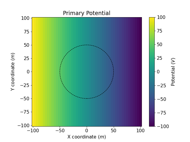
Assuming an x-directed uniform electric field and zero potential at infinity, the integration from (344) gives

(345)\[V_p = - E_0 x = -E_0 r \cos\theta\]

(Source code, png, hires.png, pdf)

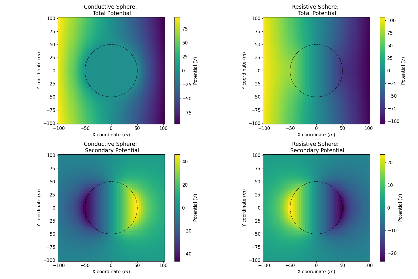
The total potential outside the sphere \((r > R)\) is

(346)\[V_1 = -E_0 \big(1 - \frac{R^3}{r^3}\frac{\sigma_1 - \sigma_0}{\sigma_1 + 2\sigma_0} \big) r \cos\theta\]

and inside the sphere \((r < R)\)

(347)\[V_2 = -E_0 \frac{3\sigma_0}{\sigma_1+2\sigma_0}r \cos\theta\]

(Source code, png, hires.png, pdf)

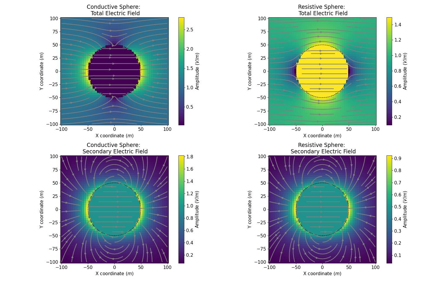
Electric Field

When an external electric field crosses conductivity discontinuities within heterogeneous media, it leads to charge buildup on the interface, which immediately gives rise to a secondary electric field governed by Gauss’s Law, to oppose the change of the primary field. Considering that the electric field is defined as the negative gradient of the potential, according to (346) and (347), the electric field at any point (x,y,z) is

(348)\[E_1 = E_0\mathbf{\hat{x}} + E_0\frac{\sigma_1-\sigma_0}{\sigma_1+2\sigma_0}\frac{R^3}{r^5}\big[(2x^2 - y^2 - z^2)\mathbf{\hat{x}} + (3xy)\mathbf{\hat{y}} + (3xz)\mathbf{\hat{z}}\big] \; (r > R)\]

(349)\[E_2 = E_0\frac{3\sigma_0}{\sigma_1+2\sigma_0}\mathbf{\hat{x}} \; (r < R)\]

(Source code, png, hires.png, pdf)

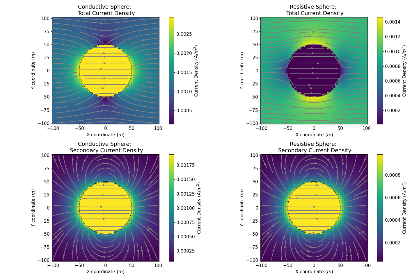
Current Density

The current density describes the magnitude of the electric current per unit cross-sectional area at a given point in space. According to Ohm’s law there is a linear relationship between the current density and the electric field at any location within the field: \(\mathbf{J} = \sigma \mathbf{E}\). This can be directly used to compute both the total and the primary current densities.

Secondary Current

The secondary current density is defined as a difference between the total current density, \(\mathbf{J_T} = \sigma \mathbf{E_T}\) and the primary current \(\mathbf{J_0} = \sigma_0 \mathbf{E_0}\)

(350)\[\begin{split}\mathbf{J_s} &= \mathbf{J_T} - \mathbf{J_0} \\ &= \sigma\mathbf{E_T} - \sigma_0 \mathbf{E_0} \\ &= (\sigma_0 + \Delta\sigma)(\mathbf{E_0} + \mathbf{E_s}) - \sigma_0 \mathbf{E_0} \\ &= \Delta\sigma\mathbf{E_0} + \sigma \mathbf{E_s}\end{split}\]

Outside the sphere, the secondary current \(\mathbf{J_s}\) acts as a electric dipole, due to and in accordance with the charge build-up at the interface (see Charge Accumulation below).

Inside a conductive sphere, \(\mathbf{J_T}\) is bigger than \(\mathbf{J_{0}}\), but in the same time \(\mathbf{E_0}\) is bigger than \(\mathbf{E_{Total}}\). The secondary current \(\mathbf{J_s}\) is in the reverse direction compared to the secondary electric field \(\mathbf{E_s}\). The boundary condition, stating that the normal component of current density is continuous, is then respected by the secondary current.

Inside a resistive sphere, \(\mathbf{J_T}\) is smaller than \(\mathbf{J_{0}}\) but in the same time \(\mathbf{E_0}\) is smaller than \(\mathbf{E_{Total}}\). The secondary current \(\mathbf{J_s}\) is again in the reverse direction compared to the secondary electric field \(\mathbf{E_s}\) and the boundary condition for the normal component of current density is respected.

This can seem counter-intuitive at first as, inside the sphere, the secondary current go from the negative to the positive charges (see Charge Accumulation below). However we can explain it by saying that the current inside the sphere is building the charges and not the reverse.

(Source code, png, hires.png, pdf)

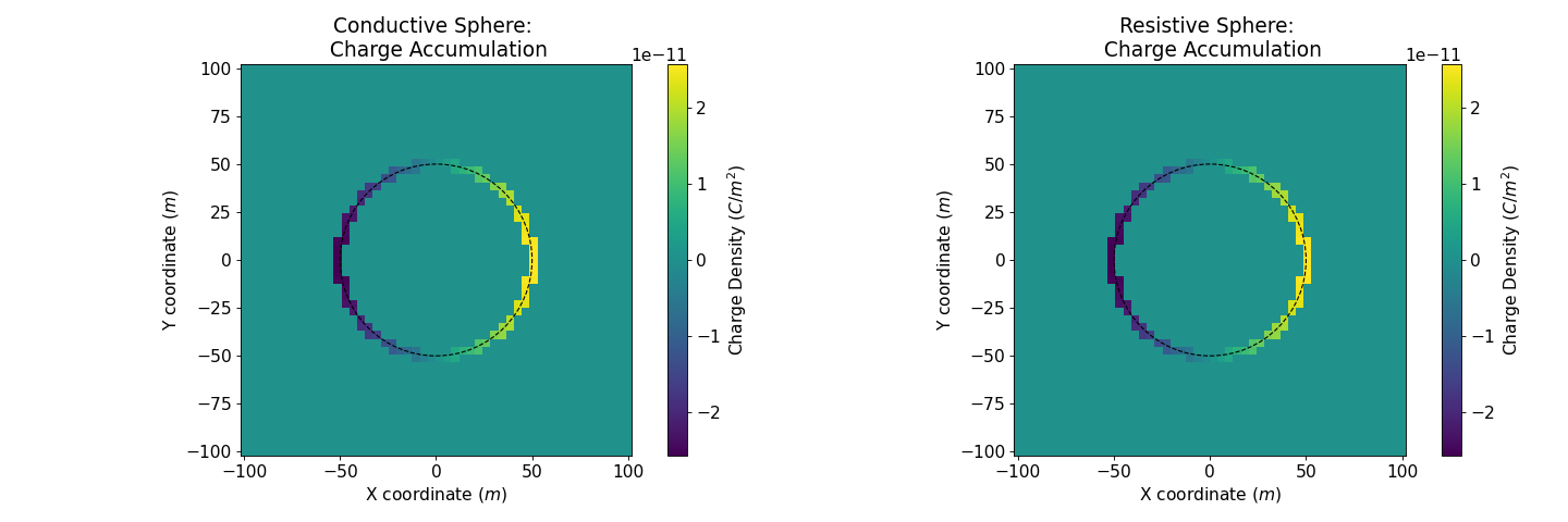
Charge Accumulation

Conductivity discontinuities will lead to charge buildup at the boundaries of these discontinuities. According to Gauss’s Law for Electric Fields, the electric charge accumulated on the surface of the sphere can be quantified by

(351)\[\int_V \boldsymbol{\nabla} \cdot \mathbf{e} \; \mathrm{d}V = \int_V \frac{\rho}{\varepsilon_0} \mathrm{d}V = Q\]

Based on Gauss’s theorem, surface charge density at the interface is given by

(352)\[\mathbf{e}_1 \cdot \mathbf{n} - \mathbf{e}_2 \cdot \mathbf{n} = \frac{\rho_s}{\varepsilon_0}\]

According to (348) (349), the charge quantities accumulated at the surface is

(353)\[\oint_S \rho_s \mathrm{d}a = \varepsilon_0 \oint_S (\mathbf{e}_{1n} - \mathbf{e}_{2n}) = \varepsilon_0 \oint_S 3\mathbf{E_0} R^2 \frac{\sigma_1-\sigma_0}{\sigma_1 + 2\sigma_0}\cos\theta \sin\theta \mathrm{d}\phi\mathrm{d}\theta\]

The figure below shows surface charge density at the surface of sphere.

(Source code, png, hires.png, pdf)

Data

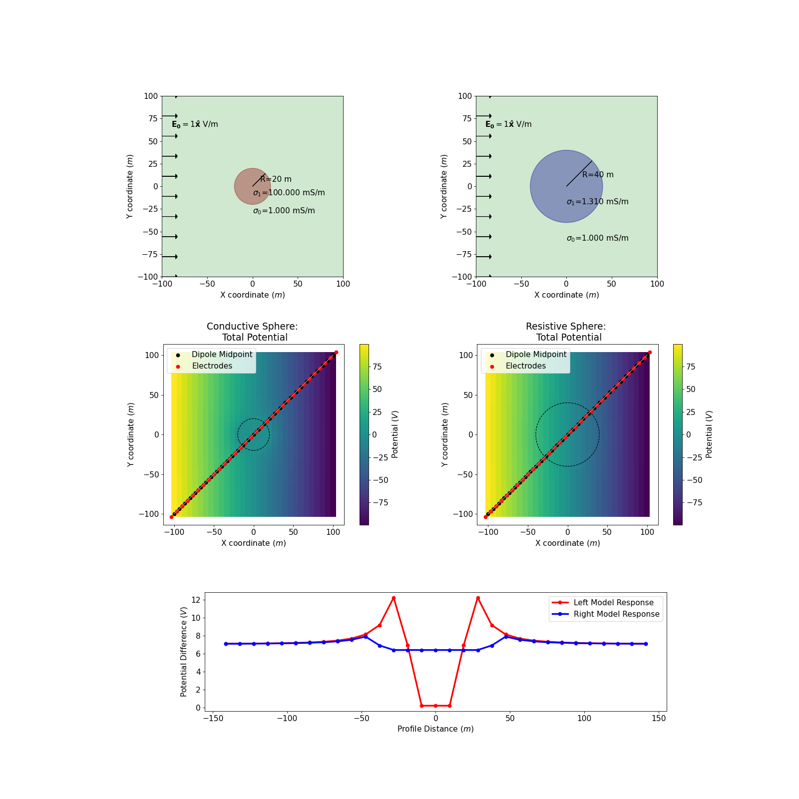
During a DC survey, we measure the difference of potentials between two electrodes, often along a profile.

Therefore, when we look at data (as in the bottom plot), we see that they will depend upon the orientation of the survey line, as well as the spacing between electrodes.

We also notice that the differences measured inside the sphere are constant, whereas outside the sphere, we observe variations in the potential differences in the vicinity of the sphere that then approach a constant value as we move away from the sphere.

For a conductive sphere, the potential differences measured in the area of influence of the sphere are smaller than the background. This can be anticipated using Ohm’s law. The reverse is observed for a resistive sphere.

(Source code, png, hires.png, pdf)

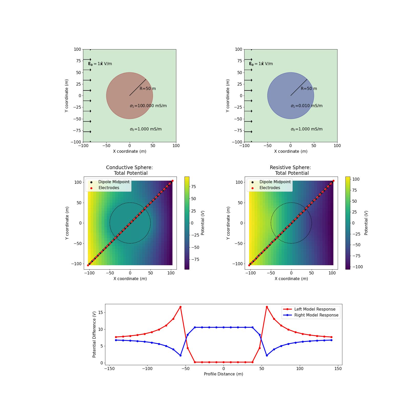
Building some Intuition for DC problem

In real life, we do not know the underground configuration. We only see the data and we are trying to model the subsurface based on it. There are several sets of parameters that can fit the data perfectly. Even in the simple case presented here, where we know that the object is a sphere, whose response can be calculated analytically, we find several configurations that can produce the same data along the same profile.

Here is an example of two spheres generating the response along the chosen profile. The only parameters that have changed are the radius and the conductivity of the sphere.

(Source code, png, hires.png, pdf)