Effects of Topography

For this derivation, we will examine the effects of negative topography by considering a hemispherical depression in the Earth’s surface.

This builds upon the solution for Point current source and a conducting sphere. By setting the resistivity of the sphere to infinity, and by exploiting the symmetry, the solution for a hemispherical depression within a halfspace is presented.

Electric Potential Across a Hemispherical Depression in a Conducting Half-Space

Here, we consider the electric scalar potential at \(P\), which results from the injection of current near a hemispherical depression of radius \(a\), centered at (\(0,0,0\)). According to Telford, so long as current is being injected along the axis of symmetry shown in Fig. 82, and \(x_0>a\), we can obtain our solution from Eq. (363) by replacing \(4\pi\) with \(2\pi\); replacement of the constant is done because all current flows entirely through the ground. By setting \(\rho_1 = \infty\), the potential created by the injection of current \(I\) at (\(x_0,0,0\)) is:

(363)\[\phi (r, \theta, \phi) = \frac{I\rho}{2 \pi} \Bigg [ \frac{1}{R} + \sum_{n=0}^\infty \frac{a^{2n+1}}{\big (x_0 \, r \big )^{n+1}} \Bigg ( \frac{n}{n+1} \Bigg ) P_n \big ( cos \theta \big ) \Bigg ]\]

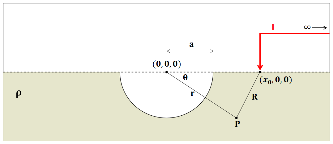
Fig. 82 Diagram showing the setup for computing the potential due to a halfspace with a hemispherical depression with a pole source.

Recall that at this point, \(x_0\) is the radial distance from the origin, within a spherical coordinate system relative to the axis of symmetry. Using Eq. (364) however, we can solve the problem in Fig. 83, where a current of \(I\) is being injected at \((x_1,\pi,0\)) and a current of \(-I\) is being injected at (\(x_2,0,0\)):

(364)\[\begin{split}\begin{split} \phi (r , \theta, \phi) &= \phi_{+} + \phi_{\, -}\\ &= \frac{\rho I}{2 \pi} \Bigg [ \frac{1}{R_1} - \frac{1}{R_2} + \sum_{n=0}^\infty \Bigg ( \frac{n}{n+1} \Bigg ) \Bigg ( \frac{a^{2n+1} P_n \big ( cos \theta_1 \big ) }{\big (x_1 \, r \big )^{n+1}} - \frac{a^{2n+1} P_n \big ( cos \theta_2 \big ) }{\big (x_2 \, r \big )^{n+1}} \Bigg ) \Bigg ] \end{split}\end{split}\]

where, by the cosine law:

\[R_1 = \sqrt{x_1^2 + r^2 - 2r x_1 cos \theta_1 \;}\]

and

\[R_2 = \sqrt{x_2^2 + r^2 - 2rx_2 cos \theta_2 \;}\]

It is important to note that Eq. (364) is only possible if current is being injected along the axis of symmetry. In addition, \(\theta\) refers an azimuthal angle relative the axis of symmetry, whereas \(\theta_1\) and \(\theta_2\) are strictly angles related to the trigonometry of the problem.

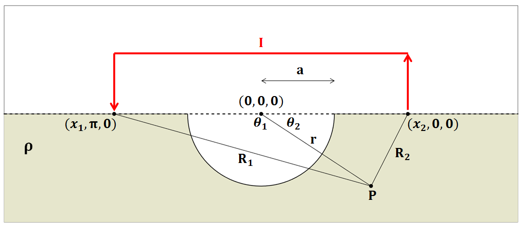
Fig. 83 Diagram showing the setup for computing the potential due to a halfspace with a hemispherical depression with a dipole source.

Examples

Using the depressed hemi-sphere solution for DC problem, we want to identify effects of topography in terms of two aspects:

• Numerical accuracy of 3D DC forward modelling algorithm (UBC DCIP3D)

• Understanding charge-build up and corresponding electrical fields

First item is important since we use this forward modelleing algorithm for the inversion of DC data. If this topographic effect is not accurately computed, then this will generate artifacts in the recovered resistivity model. In addition, if the numerical and analytic solution show a compatible match, this will provide with us cross-checks for both numerical and analytic solutions.

Note

There can be errors on derived analytic solutions!

Without a physical understanding of electromagnetic fields in the earth, the proper use of EM geophysics is difficult, thus it is important to develop a thorough understanding of electromagnetic theory. To investigate effects only due to topography, we subtract the primary potential (\(\phi^p = \frac{I\rho}{2\pi R}\)) from the total potential, \(\phi\) which yields the secondary potential (\(\phi^s\)):

\[\phi^s = \phi - \phi^p\]

By taking the gradient, then the electric field \(\bf{e}\) and total charge density (\(\rho_T\)) can be computed using equations below:

(365)\[\bf{e}=-\nabla \phi\]

(366)\[\rho_T = \epsilon_0 \nabla \cdot \bf{e}\]

Observations of total, primary, and secondary electric fields and charge density will provide us with a comprehensive understanding of topographic effects in the DC problem.

Numerical validations

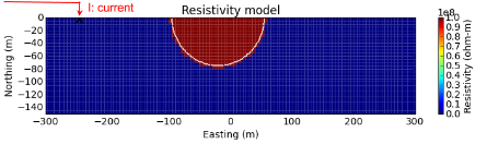
Fig. 84 Section view of 3D resistivity model for depressed hemi-sphere.

The above resistivity model shows a depressed hemisphere model. The resistivity of the depressed hemi-sphere is set to \(10^8\) ohm-m (close to infinity) to simulate air, and the half-space is set to and \(10^3\) ohm-m. To compute potentials from the above depressed hemi-sphere model, we first use numerical solutions using DCIP3D code [OL94b]. Then to check the accuracy of our numerical algorithm we use analytic solution of a sphere problem that we derived in Section Electric Potential Across a Hemispherical Depression in a Conducting Half-Space. If you want to see the numerical code used for evaluating the analytic solution See DC sphere code. To proceed with this validation, we consider a pole transmitter injected in the ground. In the above figure, injected current source location is shown.

For numerical computations, a 3D mesh with 5 m core cells is used. We compute potentials in every cells in the 3D domain. Top and middle panels of the below figure shows computed numerical and analytic potentials, respectively. White lines delineate the boundary of the depressed hemi-sphere. The bottom panel of below figure shows relative error, and blank region close to the source has errors greater than 10 percent. Even at the boundary of the hemi-sphere, we have less than 4 percent error. This is a reasonable accuracy considering that our noise level is roughly 10 percent for the DC problem. This shows our numerical solution has a capability to accurately compute those topographic effects, although our choice of discretization is clearly important.

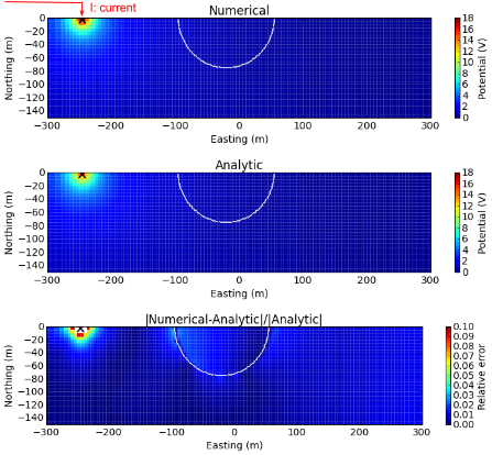
Fig. 85 Comparisons of numerical and analytic total potentials with topography. White line depicts the boundary of the depressed hemisphere.

For a more careful observation, we provide a similar comparison for the secondary potential in 3D space. The top, middle and bottom panels of the below figure correspondingly show numerical, analytic, and absolute errors of secondary potentials. The maximum error occurs at the hemi-sphere boundary close to the current source, but it is less than 20 percent.

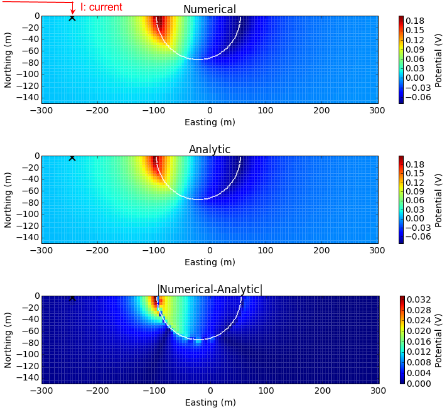
Fig. 86 Comparisons of numerical and analytic secondary potentials with topography. White line depicts the boundary of the depressed hemisphere.

Interpretations

Using Eqs. (365) and (366), we can compute both electric fields and charge density in 3D. First, we consider charge density. The below figure shows total, primary, and secondary charge densities. From the total and primary charge densities (top and middle panels), we clearly see secondary charge build-up due to the topographic effects is difficult to be recognized because of positive charges due to the input current. The secondary charge density clearly shows the topographic effects. Positive and negative charges are built up on the left side of the depressed hemi-sphere, closest to the input current. Since the air region are act as an insulator, all positive charge cannot pass through this hemi-sphere region and accumulated on the left side closer to the input current. The magnitude of negative charge build-up on the right side is much smaller than the positive charge on the other side. These positive and negative charges will generate electric fields based on Coulomb’s law (See Section Equivalence of Gauss’ Law for Electric Fields to Coulomb’s Law).

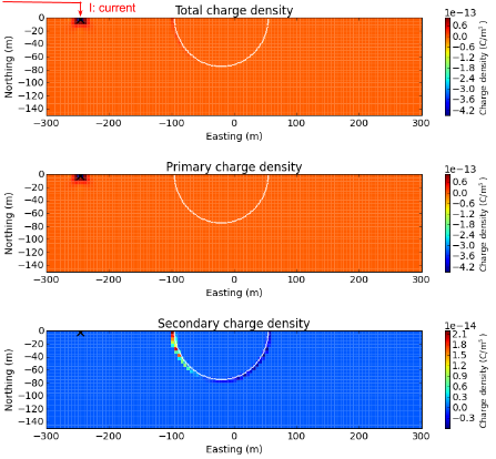
Fig. 87 Section views of total (top panel), primary (middle panel), and secondary (bottom panel) charge densities.

A rule of thumb for understanding electric fields from charges is:

Note

The electric field is coming out from a positive charge and coming into negative charge.

Based on the above principle, first imagine how electric fields are going to be distributed in 3D, then check your conjecture with the figure below, which shows total, primary, and secondary electric fields. From the total electric field shown in the top panel, we recognize that the dominant electric field is due to injected current, although we can recognize the distortion of electric fields due to charge build-up at the hemi-spherical boundary. By subtracting the primary from the total electric field we obtain a secondary electric field as shown in the bottom panel. Outside of the hemi-sphere, the electric field is dipolar in shape, while inside the hemi-sphere, the electric fields flow straight from the positive to negative charges.

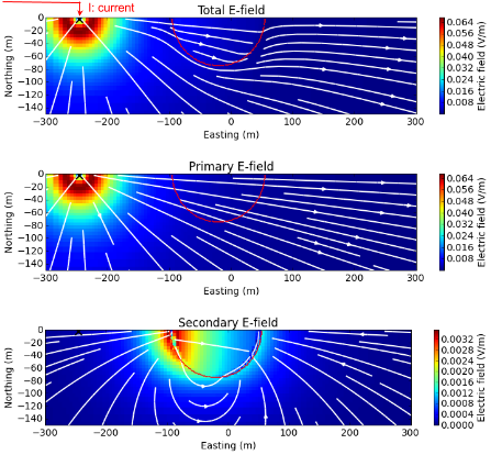
Fig. 88 Section views of total (top panel), primary (middle panel), and secondary (bottom panel) electric fields.