Through a series of experiments in 1831 Michael Faraday came to the
realization that changing magnetic fields create electric fields. Two years
later, Heinrich Lenz formulated Lenz’s Law, which characterizes the direction
of the currents induced in a conductor by these time varying magnetic fields.
A convenient way to quantify the strength of the magnetic field in a
particular region is the magnetic flux (\(\Phi_{\mathbf{B}}\)),
shows that any variation in the magnetic flux produces an electromotive force
(emf, \(\mathcal{E}\)). This emf creates electrical currents within those
bodies which are subjected to the time varying flux. The amplitude of the
induced current is dependent on the strength of the emf and the conductivity
of the material, while the direction of the induced current is characterized
by Lenz’s Law.
Lenz’s Law states that the induced current will flow in such a direction that
its secondary or induced magnetic fields act to oppose the observed change in
magnetic flux. Simply put, “nature abhors a change in flux” so the induced
current flows in such a manner to cancel out the change [Gri99]. This is
the reason for the negative sign in Faraday’s Law, equation
(74). Fig. 37 and the demonstration
linked below provide visual illustrations of Lenz’s Law.
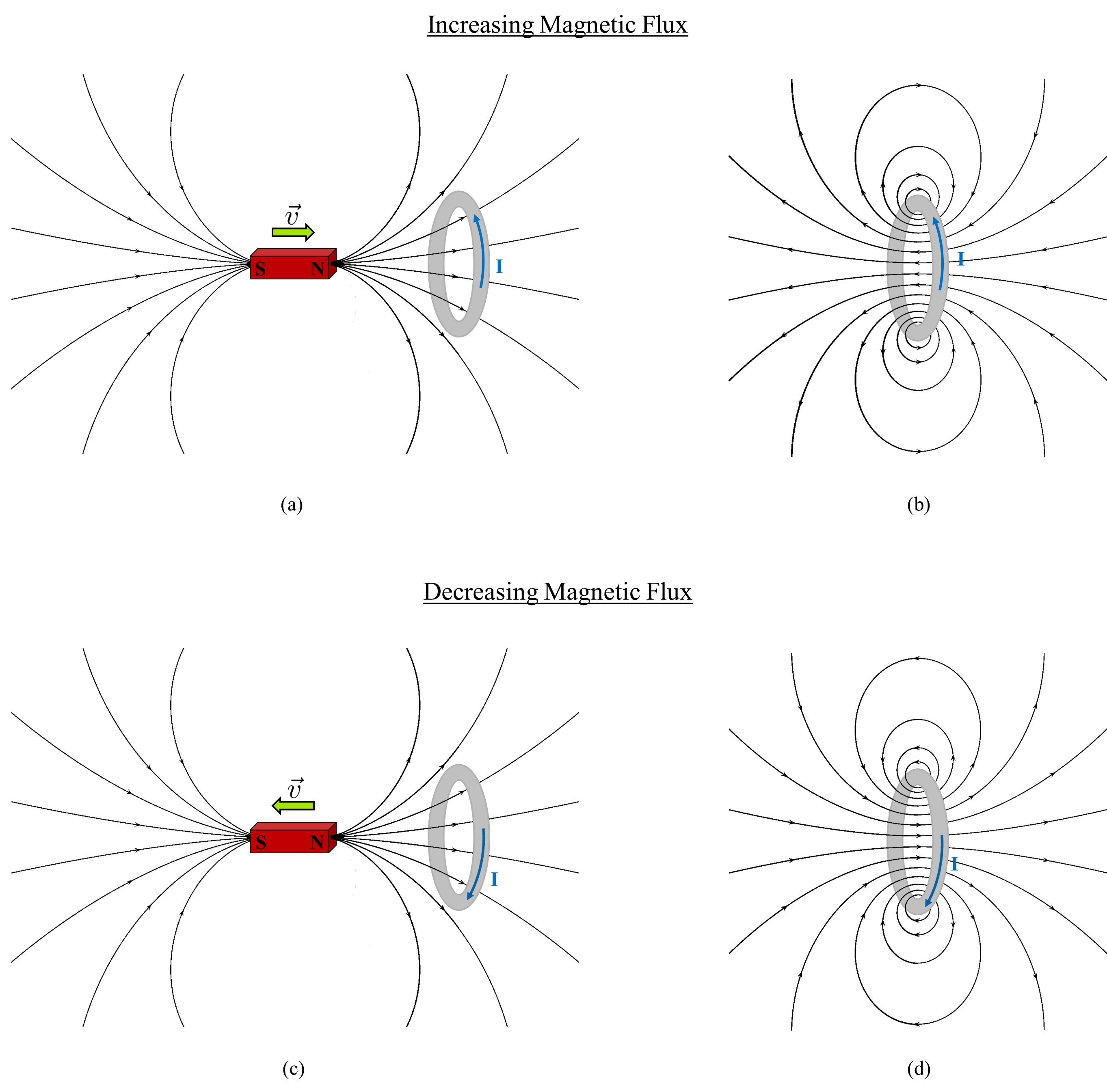
Fig. 37 In panel (a) we see a situation in which the magnetic flux through the
loop is increasing as a function of time. The induced current direction
and the secondary magnetic field which opposes the increase in flux are
shown in panel (b). Similarly, panel (c) shows when the magnetic flux
through the loop is decreasing as a function of time and panel (d)
demonstrates the direction of the induced current and secondary magnetic
field. (Figure was created by M. Mitchell using the following Wikimedia
Commons images: VFPt_dipole
and VFPt ringcurrentNoLoop
both of which are licensed under Creative Commons Attribution-Share Alike 3.0
Unported.)
Illustrative Demo:
Thanks to the Technical Services Group (TSG) at MIT’s Department of Physics
for this great demo!