Dipole Sources in Homogeneous Media
Purpose
In this section of EM GeoSci, you will learn about dipole sources and the fields they generate in homogeneous media. For each dipole source:
A physical model is supplied and used to formulate the corresponding source term in Maxwell’s equations.
Analytic expressions for the electric field, magnetic field and vector potential are then provided in both the frequency domain and time domain.
Asymptotic expressions are provided for several cases.
Numerical modeling tools are made available for investigating the dependency of the electric and magnetic fields on various parameters.
Introduction
Dipole sources are fundamental electromagnetic sources which exist at a single point in space. Although true dipole sources do not exist in nature, they do very well at approximating the electromagnetic sources used for many geophysical applications. In geophysics, there are two types of dipole sources: electrical current dipole sources and magnetic dipole sources.
In matter, the electrical current dipole (\(\mathbf{p}\)) generates a primary current density in the surrounding region; free current does not flow in free-space. This is illustrated in Fig. 64 (left). A magnetic dipole, on the other hand, generates a primary magnetic field in the surrounding region. This is illustrated in Fig. 64 (right). Notice how the field lines converge at a single point in space for either source. We will discuss the secondary electric and magnetic fields generated by each dipole in the subsequent material.
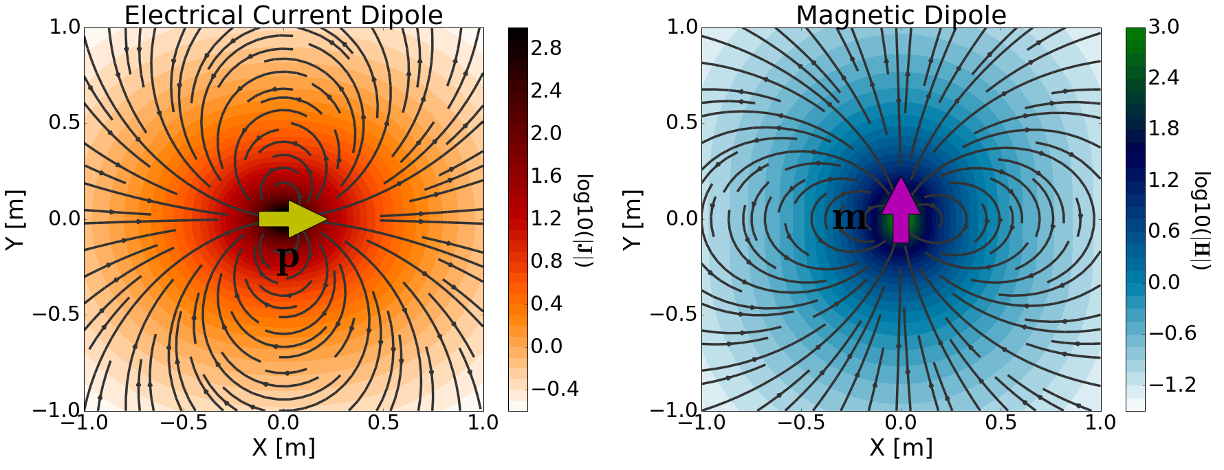
Fig. 64 (Left) Electrical current dipole ( \(\mathbf{p}\)) oriented in the \(\hat x\) direction and the primary current density ( \(\mathbf{J}\)) it produces. (Right) Magnetic dipole ( \(\mathbf{m}\)) oriented in the \(\hat y\) direction and the primary magnetic field ( \(\mathbf{H}\)) it produces.
Both electrical current dipoles and magnetic dipoles can be represented as source terms in Maxwell’s equations. For the electrical current dipole, the source term (\(\mathbf{J_e^s}\)) represents an electrical current density and has units A/m \(\!^2\). For the magnetic dipole, the source results from a magnetization (\(\mathbf{M}\)). However, the magetic source term (\(\mathbf{J_m^s} = - i\omega \mu \mathbf{M}\)) is generally represented by a magnetic current density, where \(\mathbf{J_m^s}\) has units V/m \(\!^2\). Details regarding the electric and magnetic current densities were provided along with the Ampere-Maxwell equation.
In the presence of an electromagnetic source, Maxwell’s equations in the frequency domain are given by:
where \(\pm\) depends on a choice in sign convention. Equivalently, Maxwell’s equations in the time domain are given by:
where \(\mathbf{j_e^s}\) and \(\mathbf{j_m^s}\) are time-dependent electric and magnetic source terms, respectively. Ultimately, the right-hand side of Faraday’s law becomes non-zero in the presence of a magnetic source. And the right-hand side of the Ampere-Maxwell law becomes non-zero in the presence of an electrical current source.
Organization
For each dipole source, we begin by presenting a physical model. This is used to replace frequency-dependent or time-dependent source terms in Maxwell’s equations. Analytic and asymptotic expressions along with numerical modeling tools are then provided. Quick links to subsequent content are given below.
Electrical Current Dipole
Magnetic Dipole