Defining the Magnetic Dipole
Purpose
Here, we provide a physical description of the magnetic dipole. This is used to develop a mathematical expression which can be used to replace the magnetic source term in Maxwell’s equations.
General Description
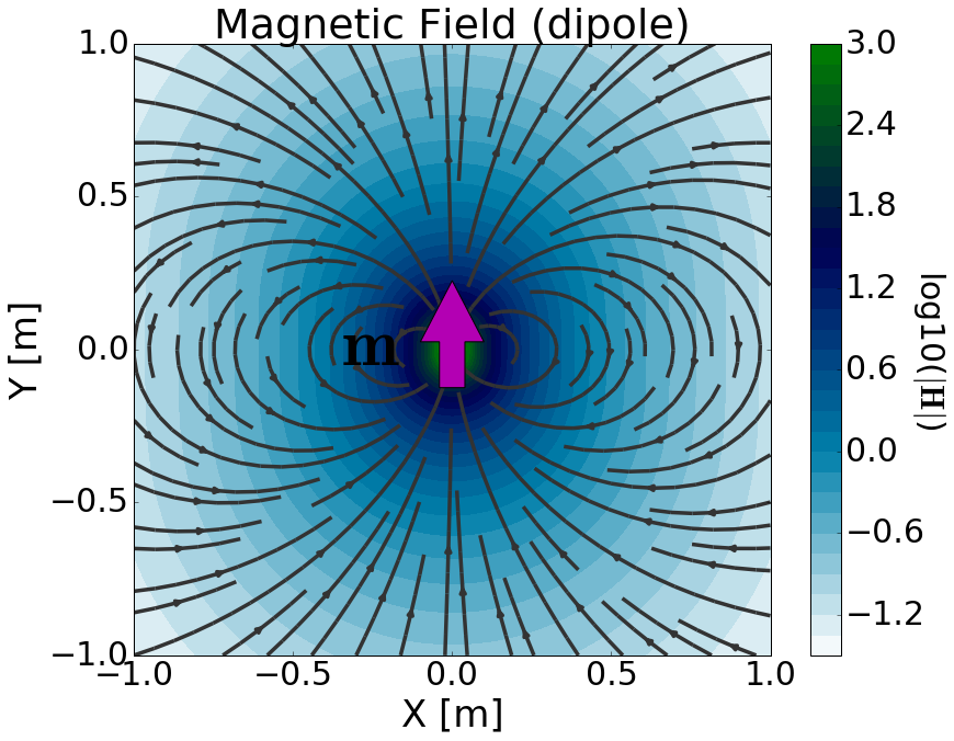
Fig. 70 Physical representation of the magnetic dipole source where \(\mathbf{m}\) = 1 Am \(\!^2\).
There are two commonly used models for the magnetic dipole. The first model describes the magnetic dipole as an infinitessimally small volume of magnetized material (i.e. a very small bar magnet). The second model describes the magnetic dipole using an infinitessimally small current loop. In both cases, the strength of the magnetic dipole source is defined by a dipole moment (\(\mathbf{m}\)). This leads to a magnetic source term (\(\mathbf{J_m^s}\)) of the form:
where \(\delta (x)\) is the Dirac delta function. The magnetic dipole source is responsible for generating a primary magnetic field in the surrounding region; secondary electric and magnetic fields are discussed later. This is illustrated in Fig. 70.
Magnetized Volume Model
This model derives the magnetic dipole source by considering a volume of uniformly magnetized material; in other words, a bar magnet. Let us assume the volume has uniform magnetization (\(\mathbf{M}\)) and has dimensions \(\Delta x\), \(\Delta y\) and \(\Delta z\); giving it a volume of \(\Delta V\). The resulting magnetic source term (\(\mathbf{J_m^s}\)) is given by:
where
and \(u(x)\) is the unit step function. Recall that \(\mathbf{J_m^s}\) defines a magnetic current density and has units V/m \(\!^2\). Thus \(\mathbf{J_m^s}\) can be used to replace the magnetic source term in Maxwell’s equations for a uniformly magnetized block.
In Fig. 71, we consider a uniformly magnetized volume where \(\mathbf{M} = M\mathbf{\hat y}\). As we can see, the magnetization contained within the volume generates a primary magnetic field in the surrounding region. Notice how the field lines seem to begin at the north end of the magnetized volume and terminate at the south (Fig. 71 left). However, when the volume is much smaller than the scale of observation (\(\Delta x, \Delta y, \Delta z \ll r\)), then it appears as though the magnetic field lines converge at a single point; see Fig. 71 (right).
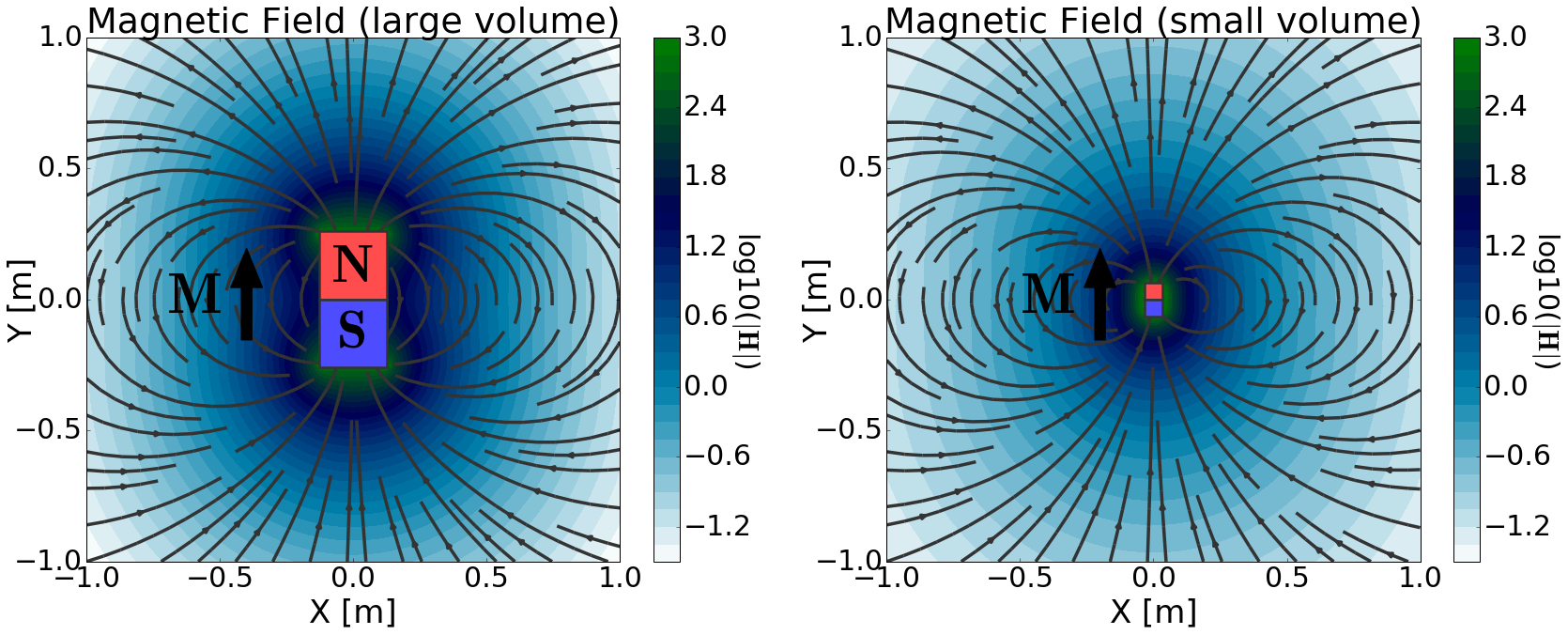
Fig. 71 Magnetic field due to a uniformly magnetized volume. Large volume (left). Small volume (right). For both volumes, the magnetization was adjusted such that \(M \Delta V\) = 1 Am \(\!^2\).
Magnetic dipoles can be used to approximate fields due to very small magnetized volumes when the scale of observation is sufficiently large. This accomplished by defining a source term which exists at a single point in space. From the previous expression, the magnetic dipole source is obtained by letting \(\Delta x , \, \Delta y , \, \Delta z \rightarrow dx, \, dy , \, dz\) ; in other words by letting \(\Delta V \rightarrow dV\). Thus the source term for a magnetic dipole is given by:
The strength of the magnetic dipole source is defined by its dipole moment (\(\mathbf{m}\)). As we can see from the previous expression, the source term depends on the product \(\mathbf{M} dV\). Thus the dipole moment which defines the magnetic dipole source is given by:
From our definition of the magnetic dipole, \(\mathbf{m}\) has units Am \(\!^2\). Each Dirac delta function carries units m \(\!^{-1}\), \(\omega\) has units s \(\!^{-1}\) and \(\mu\) has units H/m. Where 1 H = 1 V \(\!\cdot\!\) s/A, the magnetic source term (\(\mathbf{J_m}\)) has units V/m \(\!^2\).
For a magnetized rectangular block (Fig. 71 left), the magnetic field outside the source region can be calculated according to Sharma (1966); a cleaner formulation can be found in Varga. By taking the limit as \(\Delta x , \, \Delta y , \, \Delta z \rightarrow dx, \, dy , \, dz\), the magnetic field generated by a magnetized rectangular block reduces to (Fig. 71 right):
Current Loop Model
Magnetic fields are generated by the movement of electrical charges (i.e. electric current). Because of this, a magnetized volume in itself does not represent a physical source. Here, we will demonstrate how the magnetic dipole moment can be represented by an infinitessimally small loop of current.
First, let us consider a large circular loop of current with radius \(a\) and current \(I\) (Fig. 72 left). To obtain the primary magnetic field from the loop, we can use the Biot-Savart law:
The analytic solution for the Biot-Savart law in this case is rather complicated and contains several elliptic integral functions; for solution see here (link). If the radius of the loop is much smaller than the scale of observation (\(a \ll r\)), then the primary magnetic field due to the loop can be simplified to:
where \(\mathbf{\hat n}\) is the unit vector normal to the area within the loop. The primary magnetic field for a small loop is shown in Fig. 72 (right).
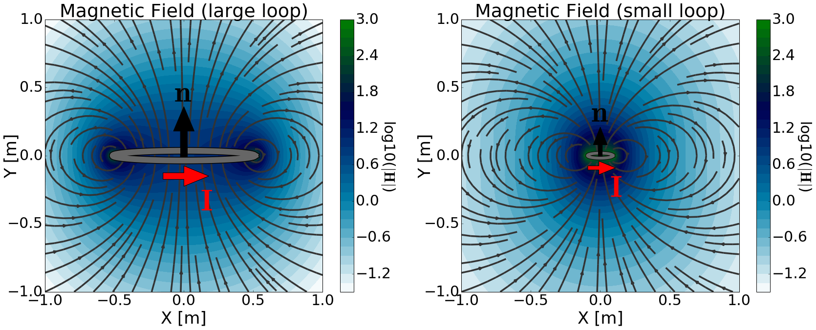
Fig. 72 Magnetic field due to a loop of current. Large current loop (left). Small current loop (right). For both loops, the current is adjust such that \(IS\) = 1 Am \(\!^2\).
Notice how the primary field for a small loop is effectively identical to that of a magnetic dipole source. Additionally, the strength of the field depends on the product of loop’s current and its area (\(S = \pi a^2\) ). Therefore, if we define the dipole moment of the loop as:
where \(\mathbf{S} = \pi a^2 I \mathbf{\hat n}\), then the primary magnetic field due to a small current loop is given by:
The previous expression tells us that if the scale of observation is significantly larger than the radius of the loop, then the loop can be represented by a magnetic dipole source. It must also follow that the loop can be represented by a corresponding magnetic dipole source term (\(\mathbf{J_m^s}\)) equal to:
Here, we have chosen a very simple treatment of the current loop model for a magnetic dipole source. A more thorough derivation of the dipole moment from Maxwell’s equations can be found in Griffiths ([Gri99]).