Ampere-Maxwell

The Ampere-Maxwell equation relates electric currents and magnetic flux. It describes the magnetic fields that result from a transmitter wire or loop in electromagnetic surveys. For steady currents, it is key for describing the magnetometric resistivity experiment.

Integral Equation

The Ampere-Maxwell equation in integral form is given below:

(62)\[\int_S \boldsymbol{\nabla} \times \mathbf{b} \cdot \mathbf{da} = \oint_C \mathbf{b} \cdot \mathbf{dl} = \mu_0 \left( I_{enc} + \varepsilon_0 \frac{d}{dt} \int_S \mathbf{e} \cdot \hat{\mathbf{n}} ~\text{da} \right),\]

where:

• \(\mathbf{b}\) is the magnetic flux

• \(\mathbf{e}\) is the electric field

• \(I_{enc}\) is the enclosed current

• \(\mu_0\) is the magnetic permeability of free space

• \(\varepsilon_0\) is the electric permittivity of free space

• \(\hat{\mathbf{n}}\) is the outward pointing unit-normal

Fig. 35 Enclosed current.

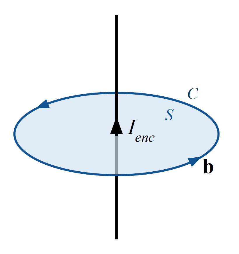
The first term of the right hand side of the equation was discovered by Ampere. It shows the relationship between a current \(I_{enc}\) and the circulation of the magnetic field, \(\mathbf{b}\), around any closed contour line (See Fig. 35). \(I_{enc}\) refers to all currents irrespective of their physical origin.

The second portion of the equation is Maxwell’s contribution and shows that a circulation of magnetic field is also caused by a time rate of change of electric flux. This explains how current in a simple circuit involving a battery and capacitor can flow. The term is pivotal in showing that electromagnetic energy propagates as waves.

Fig. 36 Integration over a capacitor

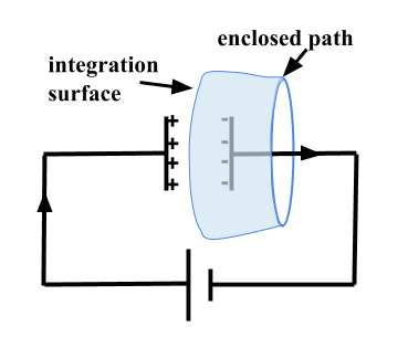
For example, imagine integrating over a surface associated with a closed path such as the one showed in Fig. 36. We can define the surface to be the area of the circle, as in Fig. 35, or alternatively, as a stretched surface, as shown in Fig. 36. In the first case, the enclosed current is the flow of charges in the wire. In the second case, however, there are no charges flowing through the surface, yet the magnetic field defined on the enclosing curve, \(C\), must be the same. This apparent discrepancy is reconciled if we take into account the displacement current, which is the time rate of change of the electric field, between the two plates. This integration is the same as if we were integrating over a flat surface with the current wire crossing it.

The integral formulations are physically insightful and closely relate to the experiments that gave rise to them. They also play a formative role in generating boundary conditions for waves that propagate through different materials.

When dealing with the propagation of EM waves in matter the currents \(I_{enc}\) are usually dealt with in terms of current densities. The integral equation above is thus written as

(63)\[\int_S \boldsymbol{\nabla} \times \mathbf{b} \cdot \mathbf{da} = \oint_C \mathbf{b} \cdot \mathbf{dl} = \mu_0 \left(\int_S \left(\mathbf{j_f} + \frac{\partial \mathbf{p}}{\partial t} + \boldsymbol{\nabla} \times \mathbf{m}\right)\cdot \mathbf{da} + \varepsilon_0 \frac{d}{dt} \int_S \mathbf{e} \cdot \mathbf{\hat{n}} ~\text{da}\right),\]

where the current densities are:

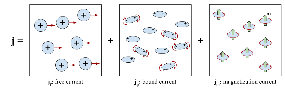
• \(\mathbf{j_f}\) is the free current caused by moving charges

• \(\mathbf{j_p} = \frac{\partial \mathbf{p}}{\partial t}\) is the polarization or bound current, where \(\mathbf{p}\) is the electric polarization resulting from bound charges in dielectrics

• \(\mathbf{j_m} = \nabla \times \mathbf{m}\) is the magnetization current, that is, the currents needed to generate the magnetization \(\mathbf{m}\)

The total current density is the sum of these three contributions and is described by

(64)\[\mathbf{j} = \mathbf{j}_f + \mathbf{j}_p + \mathbf{j}_m.\]

Note

The total current involved in the Ampere-Maxwell equation consists of free current and bound current, although all currents are essentially the same from a microscopic perspective. Treating free current and bound current differently offers physical insights to the Ampere-Maxwell equation in different contexts.

The free current is caused by moving charges which are not tied to atoms, often referred to as conduction current. In contrast, the bound current is induced by a magnetization or a polarization in bulk materials. When a magnetic material is placed in an external magnetic field, a magnetization current will be induced due to the motion of electrons in atoms. Likewise, when an external electric field is applied to a dielectric material, the positive and negative bound charges within the dielectric can separate and induce a polarization current density internally.

Continuing to treat the free current and bound current separately and using the constitutive equations: \(\mathbf{b} = \mu_0(\mathbf{h} + \mathbf{m})\) and \(\mathbf{d}= \varepsilon_0 \mathbf{e} + \mathbf{p}\), the integral form Ampere-Maxwell equation can be reformulated as:

(65)\[\int_S \boldsymbol{\nabla} \times \mathbf{h} \cdot \mathbf{da} = \oint_C \mathbf{h} \cdot \mathbf{dl} = \int_S \left( \mathbf{j}_f + \frac{\partial \mathbf{d}}{\partial t} \right) \cdot \hat{\mathbf{n}} ~\text{da}.\]

Note that the bound charge due to magnetization is integrated into the magnetic field \(\mathbf{h}\), whereas the bound charge due to electric polarization is integrated into the displacement field \(\mathbf{d}\).

Differential equation in the time domain

There are a number of ways of writing the equation in differential form. Each provides its own insight. We begin by considering the differential form of equation (62) in terms of the variables \(\mathbf{e, b, p}\) and \(\mathbf{m}\):

(66)\[\boldsymbol{\nabla} \times \mathbf{b} - \varepsilon_0 \mu_0 \frac{\partial \mathbf{e}}{\partial t} = \mu_0\left( \mathbf{j_f} + \frac {\partial \mathbf{p}}{\partial t} + \boldsymbol{\nabla} \times \mathbf{m}\right)\]

and similar to (65), we can use the constitutive relations \(\mathbf{d}= \varepsilon_0 \mathbf{e} + \mathbf{p}\) and \(\mathbf{b} = \mu_0(\mathbf{h} + \mathbf{m})\) to write the differential time-domain equation in terms of the variables \(\mathbf{h, j_f}\) and \(\mathbf{d}\):

(67)\[\boldsymbol{\nabla} \times \mathbf{h} = \mathbf{j}_f + \frac{\partial \mathbf{d}}{\partial t}.\]

Differential equations in the frequency domain

We use the \(e^{i\omega t}\) Fourier Transform Convention to transfer our equations from the time domain to the frequency domain.

The equation becomes

(68)\[\boldsymbol{\nabla} \times \mathbf{H} - i \omega \mathbf{D} = \mathbf{J}_f.\]

If we deal with linear isotropic media then we have

\[\mathbf{D}(\omega)=\epsilon \mathbf{E}(\omega)\]

(69)\[\mathbf{J}_f(\omega)=\sigma \mathbf{E}(\omega)\]

and the Ampere-Maxwell equations can be written as

(70)\[\boldsymbol{\nabla} \times \mathbf{H} - \left(\sigma + i \omega \epsilon\right) \mathbf{E} = 0.\]

Units

Magnetic B-field	\(\mathbf{b}\)	T	tesla
Electric field intensity	\(\mathbf{e}\)	\(\frac{\text{V}} {\text{m}}\)	volt per meter
Electric current	\(\text{I}\)	A	ampere
Electric current density	\(\mathbf{j}\)	\(\frac{\text{A}} {\text{m}^{2}}\)	ampere per square meter
Magnetization	\(\mathbf{m}\)	\(\frac{\text{A}} {\text{m}}\)	ampere per meter
Electric polarization	\(\mathbf{p}\)	\(\frac{\text{A}\cdot \text{s}}{\text{m}}\)	ampere times seconds per square meter
Magnetic H-field	\(\mathbf{h}\)	\(\frac{\text{A}} {\text{m}}\)	ampere per meter
Electric displacement	\(\mathbf{d}\)	\(\frac{\text{C}} {\text{m}^{2}}\)	coulomb per square meter

Constants

Magnetic constant	\(\mu_0 = 4\pi ×10^{−7} \frac{\text{N}}{\text{A}^2} \approx 1.2566370614...×10^{-6} \frac{\text{T}\cdot \text{m}}{\text{A}}\)
Vacuum permittivity	\(\varepsilon_0 \approx 8.854 187 817... × 10^{−12} \frac{\text{F}}{\text{m}}\) (farads per meter)

Conversions

• One Tesla equals one weber (the SI unit of magnetic flux) per square meter:

\[1 \text{T} = 1 \frac{\text{Wb}}{\text{m}^{2}} = 1 \frac{\text{V}\cdot \text{s}}{\text{m}^{2}}.\]

• One ampere equals one coulomb (the SI unit of electric charge) per second:

\[1 \text{A} = 1 \frac{\text{C}}{\text{s}}.\]

Discovers of the law

The first observation that spurred researchers to look for the relationship linking magnetic field and current was made by Hans Christian Ørsted in 1820, who noticed that magnetic needles were deflected by electric currents. This led several physicists in Europe to study this phenomenon in parallel. While Jean-Baptiste Biot and Félix Savart were experimenting with a setup similar to Ørsted’s experiment (that lead them to define in 1820 a relationship known now as the Biot-Savart’s law), André-Marie Ampère’s experiment focused on measuring the forces that two electric wires exert on each other. He formulated the Ampere’s circuital law in 1826 [Gri99], which relates the magnetic field associated with a closed loop to the electric current passing through it. In its original form, the current enclosed by the loop only refers to free current caused by moving charges, causing several issues regarding the conservation of electric charge and the propagation of electromagnetic energy.

In 1861 [Max61], James Clerk Maxwell extended Ampere’s law by introducing the displacement current into the electric current term to satisfy the continuity equation of electric charge. Based on the idea of displacement current, in 1864 [Max65], Maxwell established the theory of electromagnetic field, predicating the wave propagation of electromagnetic fields and the equivalence of light propagation and electromagnetic wave propagation.

It was not until the late 1880s [Her93], Heinrich Hertz experimentally proved the existence of electromagnetic waves as predicated by Maxwell’s electromagnetic theory, and demonstrated the equivalence of electromagnetic waves and light.

These efforts have lain solid foundations for the development of modern electromagnetism.