Physics

Purpose

Demonstrate the fundamental physical principles governing the IP experiment

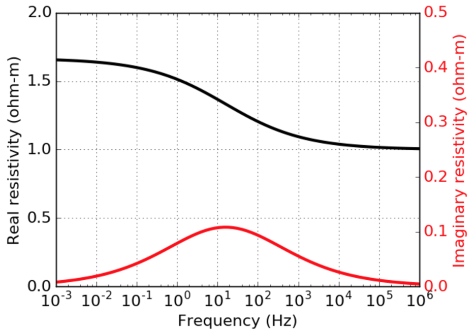
Fig. 166 Complex conductivity in frequency domain. Pelton’s Cole-Cole model [PWH+78] model is used (\(\eta\) = 0.4, \(\tau\) = 0.01 s, \(c\) = 0.4).

In the DC experiment we assumed non-dispersive electrical resistivity, i.e. not frequency-depndent. However, in reality resistivity of the earth material is dispersive, and effectively generate polarization charge buildup when electric field is applied to a chargeable medium. For instance, Fig. 166 shows complex-valued resistivity in frequency domain. They have real and imaginary parts, and vary in frequency.

To understand the impact of complex resisitivty, we only consider the end member of the resistivity at zero and infinte frequency: \(\rho_0\) and \(\rho_{\infty}\), respectively. Chargeability, \(\eta\) can be defined as

\[\eta = \frac{\rho_0-\rho_{\infty}}{\rho_0}\]

Now considering a homoegenous earth with Ohm’s law (\(V=IR\)), we redefine

(488)\[\eta = \frac{V_0-V_{\infty}}{V_0}\]

where \(V_0\) and \(V_{\infty}\) are voltages at zero and infinte frequency, respectively.

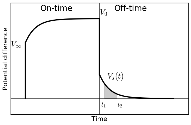
Fig. 167 Overvoltage curve in time domain.

In time domain, measured voltage will look like Fig. 167 with a half-duty cylcle current. For inhomogeneous earth medium Eq. (488) should be modifed as

(489)\[\eta_a = \frac{V_0-V_{\infty}}{V_0}\]

where \(\eta_a\) is an apparent chargeability. Therefore, in general induced polarization (IP) effects can be considered as a perturbation of voltage due to a small resistivity change. \(V_0\) is a voltage when polarization charge buildup is at maxium, and hence a voltage due to IP effects can be defined as

\[V_{IP} = V_0-V_{\infty}\]

Similarly, aribitrary IP current density and electric field can be defined as

\[\mathbf{J}_{IP} = \mathbf{J}_0-\mathbf{J}_{\infty}\]

\[\mathbf{E}_{IP} = \mathbf{E}_0-\mathbf{E}_{\infty}\]

And corresponding polarization charge density can be defined as

\[q_{IP} = \nabla \cdot \mathbf{E}_{IP}\]

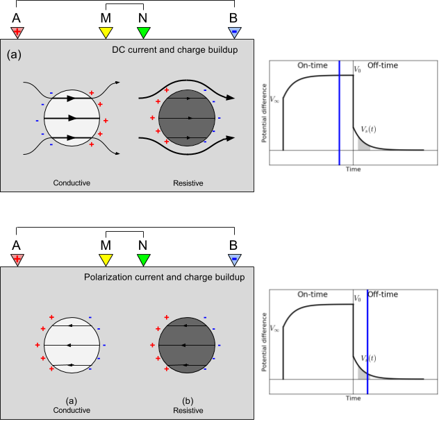
Fig. 168 DC and IP charge buildup concept.

Considering a time domain measurement, in the on-time when currents are injected, DC currents will dominate IP currents as shown in Fig. 168 hence currents are channeled into good conductors and flow around resistors; sign of charges built around the conductor and the resistor are opposite. In the off-time, DC currents are disappeared only IP currents flows, and importantly direction of IP currents are opposite to DC currents inside of both chargeable spheres resulting in same sign of charges built around both chargeable spheres. Therefore, chargeable bodies act as like a resistor.

Two-sphere problem

We illustrate the DC-IP experiment with a synthetic pole-dipole survey as illustrated in Fig. 169. This simple resistivity model is made up of two spheres in a uniform half-space Earth, and both spheres are chargeable (\(\eta\) = 100 mV/V). Currents are injected into the ground from the source, and potentials are measured at different locations. Similarly, we only consider both end members of voltage at zero and infinite frequency: \(V_0\) and \(V_{\infty}\), and by subtracting \(V_{\infty}\) from \(V_{0}\) we evaluate IP voltage, \(V_{IP}\). The source location is marked by a triangle.

Here to understand how currents flow and charges are built up in both DC and IP cases, we present both currents and charges at a vertical section crossing the center of the two spheres for each case.

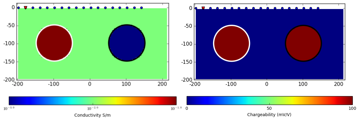
Fig. 169 Pole-dipole DC-IP experiment over a synthetic model. Right panel shows conductivity model made up of a conductive (\(10^{-1}\) S/m) and a resistive (\(10^{-3}\) S/m) sphere embedded in a uniform half-space (\(10^{-2}\) S/m). Left panel shows

DC currents and charges

As mentioned earlier, DC datum can be measured at a late on-time when DC charges dominate IP charges thus, current pathes are mostly distorted due to the conductor and resistor reflected in \(\rho_0\).

Note

[Press play] Note the behaviour of the current lines as the point source passes over the conductor. The current density increases inside the sphere but decreases around it; this is often referred to as current channeling. Conversely, current lines get deflected around the resistor.

[Pause] Charges accumulate at the interface between conductivity contrasts. Note the difference in charge polarity as the current flows into the conductive and resistive spheres. The polarities agree with those predicted by theory. Also note how the spatial distribution of charges on the spheres changes as the current source is moved.

– +

Once Loop Reflect

IP currents and charges

IP datum can be measured at an off-time when DC currents are gone. At this time only polarization charges exists resulting in IP currents and measured IP voltages.

Note

[Press play] The conductive and chargeable sphere (left) acts like dipolar currents with the opposite direction to the DC currents. The current density decreases as the distance from the sphere increases. Similar pattern of IP currents can be observed for the resistive and chargeable sphere (right), but with smaller amplitude than the other one.

[Pause] Charges accumulate at the interface between chargeability contrasts. Note the same charge polarity as the current flows into the conductive and resistive spheres (both chargable). Considering the polarity a chargeable body acts like a resistor.

– +

Once Loop Reflect