Interpretation
Purpose
To show how airborne FDEM data are processed and inverted to reveal meaningful information about the earth structure.
Interpretation is the process that extracts information in the delivered data to make decisions or to derive geologic knowledge. Depending on the specific geologic questions asked, and the resources available, geophysicists can choose from a wide spectrum of approaches ranging from trivial and low-resolution to sophisticated and high-resolution.
Preliminary interpretation
Data plotting
Significant amount of information, especially the relative distribution of conductivity, can be obtained by just plotting the data. Sometimes simple data transform techniques can also be used to isolate the anomaly and aid the interpretation. This type of approach can include: direct data plotting, data- conductivity transform, empirical template method, etc. Those simple methods were once the mainstream, but have shown drawbacks in complex geological setting and lack the ability to decode the conductivity values from the data. However, it still has its value in data quality control and preliminary interpretation.
We use a simple sphere in a halfspace model similar to the sphere in a resistive halfspace example, but this time using a larger halfspace conductivity (\(10^{-2}\) S/m). Notice that the response away from the sphere varies greatly between frequencies due to the response from the ground.
Apparent conductivity
Apparent conductivity is another semi-qualitative method that further ties the data to the conductivity of the ground. It is defined as the conductivity of a uniform half-space that would generate the same data at a particular time or frequency. It can be considered as a lumping averaging of the conductivities around the measurement location. Despite its blending effect, it provides qualitative insight about how the conductivity varies from shallow (high frequency) to deep (low frequency). In combination with a depth estimation using skin depth, apparent conductivity forms the basis of a host of imaging methods, referred to as conductivity-depth transform (CDT) or imaging (CDI).
Quantitative Inversion
1D layered earth inversion
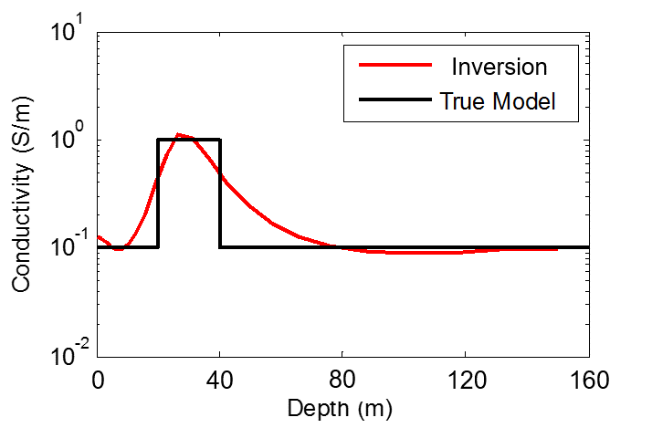
Fig. 188 1D layered earth inversion of the 3-layer model.
This approach assume the earth’s conductivity only varies as a function of depth. At each measurement location, the inversion find a layered model that explains the data at all the observing frequencies. Fig. 188 shows the 1D inversion result of the 3-layer example in Physics. The conductive layer from 20 to 40 m depth is reasonably recovered by the inversion, although the interfaces are not sharp becasue of the smooth constraint used in the inversion.
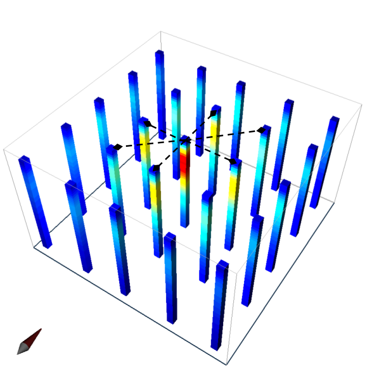
Fig. 189 1D layered earth inversions of the sphere model.
For the data from the sphere model, 1D inversion can still be performed at individual stations to provide information about local changes in conductivity. Fig. 189 presents such 1-D models in a 3-D space for the sphere example, but the lack of lateral continuity makes it difficult to interpret. Many layered models at multiple locations then can be stitched together to form a pseudo-3D volume for model visualization. Advanced techniques can also consider the correlation between adjacent locations by imposing lateral constraints.
Here we use the synthetic data set generated for the sphere model as an example to demonstrate the 1D inversion technique. The earth is horizontally divided into 20 layers from the surface to the basement. The top layer is 0.5 m thick, and the layers are gradually thickened at a rate of 1.2 toward the depth. The data are noise-free, but we assume that there is a 20 ppm noise floor in both in-phase and quadrature. The animation below compares the observed (top) and predicted (bottom) data and the pseudo-3D conductivity model obtained by stitching the individual 1D layered models. The sphere is reasonably imaged on the cross section. Although the sphere’s geometry is distorted and its conductivity value is underestimated, the inversion still reasonably reflects the correct horizontal location and the depth to the sphere’s top.
2D/3D inversion
2D/3D inversion Although the layered earth assumption in 1D inversion has provided a reasonable inversion model, the artifacts and distortion due to the 2D or 3D lateral variation of conductivity can significantly complicate the interpretation in practice. In the synthetic inversion of the sphere, the object is horizontally stretched on the cross section of the 1D stitched model, because the soundings away from the sphere can still sense the high conductivity of the sphere. The underestimated conductivity value is the result of spreading the conductive material belonging to a compact body to an infinite layer in the 1D model.
The solution to overcome the drawbacks of 1D inversion is to consider the lateral variation of conductivity by using a 2D or 3D model. A 2D/3D inversion discretizes the entire earth to many discrete cells, each of which has a constant conductivity. Then the Maxwell’s equations are numerical solved on the mesh. The obtained images of the subsurface are then in 3D voxel format. 3D inversions provides the best resolution and works for any complicated models in reality, but it is more computationally expensive. 3D inversion is a very involving topic, so we present it in another part of EM.GeoSci.