Analytic Derivation

Purpose

Here, analytic expressions for the impulse response and step-off excitation for a conductive and magnetically permeable sphere are derived. These derivations follow the ones found in Wait ([Wai51]) and Wait and Spies ([WS69]).

Introduction

According to Wait and Spies ([WS69]), the induced dipole moment \(m(t)\) characterizing a sphere’s time-dependent electromagnetic excitation is defined by a convolution:

(457)\[m(t) = \Bigg ( \frac{4\pi}{3} R^3 \Bigg ) \int_{-\infty}^\infty \chi (\tau) h_0 (t-\tau )d\tau\]

where \(R\) is the sphere’s radius, \(\chi (t)\) represents the sphere’s impulse response and \(h_0 (t)\) represents the inducing field. By definition, \(\chi (t)\) is the inverse Fourier transform of the sphere’s frequency-dependent excitation factor ([Wai51]):

(458)\[\chi (t) = \frac{1}{2\pi} \int_{-\infty}^{\infty} \chi (i \omega) e^{i\omega t} d\omega\]

However, if a change of variables is used (\(s = i\omega\)), then Eq. (458) can be more generally expressed as an inverse Laplace transform:

(459)\[\chi (t) = \frac{1}{2 \pi i} \int_{c - i\infty}^{c + i\infty} \chi (s) e^{st} ds = \mathcal{L}^{-1} \big [ \chi (s) \big ]\]

where \(\chi (s)\) is the sphere’s excitation factor parameterized in terms of a variable \(s\). A small positive constant \(c\) is chosen so that the contour path of integration lies within the convergence region of \(\chi (s)\). Here, our derivations begin with frequency-domain expressions for the sphere’s excitation factor according to Wait ([Wai51]). Next, solutions using the inverse Laplace transform are derived according to Wait and Spies ([WS69]).

Purely Conductive Sphere

Here, we derive the unit-step excitation and the impulse response for a conductive and non-permeable (\(\mu = \mu_0\)) sphere. In this case, the frequency-dependent excitation factor \(\chi (i\omega)\) for the sphere is defined by ([Wai51]):

(460)\[\chi (i\omega) = - \; \frac{3}{2} \Bigg [ 1 + \frac{3}{\alpha^2} - \frac{3 \, \textrm{coth} (\alpha)}{\alpha} \Bigg ]\]

where:

(461)\[\alpha = \Big [ i \omega \mu_0 \sigma \Big ]^{1/2} R \; ,\]

\(R\) is the radius of the sphere, \(\sigma\) is the conductivity of the sphere and \(\mu_0 = 4 \times 10^{-7}\) H/m is the permeability of free-space.

Impulse Response

To obtain the excitation factor’s impulse response, Wait and Spies ([WS69]) employed a change of variables on Eq. (460). By replacing \(s=i\omega\), letting \(\beta=(\mu_0 \sigma)^{1/2} R\) and re-expressing the hyperbolic cotanjent as an infinite series, Eq. (460) becomes:

(462)\[\begin{split}\begin{align} \chi (s)&= - \; \frac{3}{2} \Bigg [ 1 + \frac{3}{\beta^2 s} - \frac{3 \, \textrm{coth} (\beta s^{1/2} )}{\beta s^{1/2}} \Bigg ] \\ &= - \; \frac{3}{2} \Bigg [ 1 + \frac{3}{\beta^2 s} + \frac{3}{\beta s^{1/2}} \Bigg ( \frac{1 + e^{-2 \beta s^{1/2} } }{1 - e^{-2 \beta s^{1/2}}} \Bigg ) \Bigg ] \\ &= - \; \frac{3}{2} \Bigg [ 1 + \frac{3}{\beta^2 s} - \frac{3}{\beta s^{1/2}} - \frac{6}{\beta} \sum_{n = 1}^\infty \frac{e^{-2n \beta s^{1/2}}}{s^{1/2}} \Bigg ] \end{align}\end{split}\]

For each of the terms within Eq (462), the inverse Laplace transform is now trivial and can be looked up in tables. As a result, the solution to Eq. (459) is given by:

(463)\[\chi (t) = - \; \frac{3}{2} \delta (t) - \frac{9}{2} \Bigg [ \frac{1}{\beta^2} - \frac{1}{\beta \sqrt{\pi t}} \Bigg ( 1 + 2 \sum_{n = 1}^\infty e^{-(n\beta)^2/t} \Bigg ) \Bigg ] u(t)\]

where \(\delta(t)\) is the Dirac delta function. We can see that Eq. (463) is zero for \(t<0\), implying it is causal. It should be noted that our expression for \(\chi (t)\) differs from the one in Wait and Spies ([WS69]) by a factor of \(-3/2\). This is because of how we chose to define \(\chi (i\omega)\). Although the impulse response is written as an infinite series, exponential terms become negligible when the product of \((n\beta)^2t\) is sufficiently large. As a result, only a finite portion of the sum is required to approximate the response to a reasonable degree of accuracy; with more terms being required at early times.

Step Response

Consider the sphere’s response to step-excitation. At time \(t=0\), an inducing field of amplitude \(H_0\) excites the sphere. The inducing field can be expressed as:

(464)\[h_0 (t) = H_0 u(t)\]

Using Eqs. (463) and (464) to solve Eq. (457):

(465)\[m(t) = \frac{4\pi}{3}R^3 \Bigg [ \int_{-\infty}^{\infty} \chi (\tau) H_0 u(t-\tau) d\tau \Bigg ] = \frac{4\pi}{3}R^3 \Bigg [ \int_0^t \chi (\tau) d\tau \Bigg ] H_0\]

The convolution in Eq. (465) only requires integration of the impulse response from 0 to \(t\). By substituting Eq. (460) into Eq (465), we can obtain the final expression presented in Wait and Spies ([WS69]):

(466)\[\int_0^t \chi (t) d\tau = - \; \frac{9}{2} \Bigg [ \frac{1}{3} + \frac{t}{\beta^2} - \frac{2}{\beta} \sqrt{\dfrac{t}{\pi}} \Bigg ( 1 + 2 \sum_{n=1}^\infty e^{-(n\beta)^2/t} \Bigg ) + 4 \sum_{n=1}^\infty n \; \textrm{erfc}\Bigg ( \frac{n\beta}{\sqrt{t}} \Bigg ) \Bigg ] u(t)\]

where \(\textrm{erfc}(z)\) is the complimentary error function given by:

(467)\[\textrm{erfc}(z) = \frac{2}{\sqrt{\pi}} \int_z^\infty e^{-t^2} dt\]

Although a rigorous proof will not be provided here, Eq. (466) goes to 0 as \(t\) goes to infinity. Thus:

(468)\[\lim_{t\rightarrow\infty} \; \int_0^t \chi (\tau) d\tau = 0\]

This is expected given that inductive responses decay to zero after sufficient time. The response to step-off excitation may be obtained by replacing the waveform in Eq. (465). This results in the following expression:

(469)\[m(t) = \frac{4\pi}{3}R^3 \Bigg [ \int_{-\infty}^{\infty} \chi (\tau) H_0 \big [ 1 - u(t-\tau) \big ] d\tau \Bigg ] = - \; \frac{4\pi}{3}R^3 \Bigg [ \int_0^t \chi (\tau) d\tau \Bigg ] H_0\]

Comparing Eqs. (465) and (469), the response to step-on and step-off excitation behave identically and have opposing sign. The rate of decay for the step-off response is obtained by taking the derivative of Eq. (469) with respect to \(t\):

(470)\[\begin{split}\begin{align} \frac{d \, m(t)}{dt} &= \frac{4\pi}{3}R^3 \Bigg [ \int_{-\infty}^{\infty} \chi (\tau) \frac{d \, h_0 (t-\tau)}{dt} d\tau \Bigg ] \\ &= \frac{4\pi}{3}R^3 \Bigg [ - \; \int_{-\infty}^{\infty} \chi (\tau) \, H_0 \, \delta (t-\tau) d\tau \Bigg ] \\ &= - \; \frac{4\pi}{3}R^3 \, \chi (t) \, H_0 \end{align}\end{split}\]

Therefore, the rate of decay may be obtained directly if the excitation’s impulse response is known. The unit step-off response for a sphere of radius \(R\) = 10 m, for several conductivities, is shown in Fig. 143.

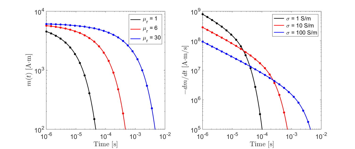
Fig. 143 Transient response for a non-permeable sphere for several conductivities.

Response from a Conductive and Magnetically Permeable Sphere in a Resistive Medium

Here we consider the time-dependent magnetization of a conductive and magnetically permeable sphere within a resistive medium (\(\sigma_b \ll \sigma\)). Expressions for the step-on response, step-off response, rate of decay, and impulse response are presented. In this case, the frequency-dependent excitation of the sphere is defined by:

(471)\[\chi (i\omega) = \frac{3}{2} \Bigg [ \frac{2\mu (\mathrm{tanh} \, \alpha - \alpha) + \mu_0 (\alpha^2 \, \mathrm{tanh} \, \alpha - \alpha + \mathrm{tanh} \, \alpha)}{\mu (\mathrm{tanh} \, \alpha - \alpha) - \mu_0 (\alpha^2 \, \mathrm{tanh} \, \alpha - \alpha + \mathrm{tanh} \, \alpha)} \Bigg ]\]

where, if electric displacement is neglected (i.e. \(\omega \varepsilon \ll \sigma\)):

(472)\[\alpha = \Big [ i \omega \mu \sigma \Big ]^{1/2} R\]

Once again, step and impulse responses for the conductive and magnetically permeable sphere can be derived using the inverse Laplace transform ([WS69]). The inverse Laplace transforms can be solved using the pole-residue theorem. As this derivation is somewhat more technical, only the final results from Wait and Spies are provided here.

Step Response

For a conductive and magnetically permeable sphere, it is easier to begin by presented expressions for the step response. According to Eqs. (457) and (459), the time-dependent excitation of the sphere can be expressed as:

(473)\[m(t) = \frac{4\pi}{3}R^3 \mathcal{L}^{-1} \big [ \chi(s) H_0 (s) \big ]\]

where \(H_0 (s)\) is the Laplace transform of \(h_0 (t)\). For a step-on excitation:

(474)\[\mathcal{L}^{-1} \big [ \chi(s) H_0 (s) \big ] = \frac{H_0}{2\pi i} \int_{c-i\infty}^{c+i\infty} \frac{\chi (s)}{s} e^{st} ds\]

where \(H_0\) is the amplitude of the step waveform and \(H_0 (s) = H_0/s\). By solving the inverse Laplace transform, the time-dependent response to step excitation is given by ([WS69]):

(475)\[m(t) = \frac{4\pi}{3}R^3 \, H_0 \Bigg [ \frac{3}{2} \Bigg ( \frac{2 (\mu_r - 1)}{\mu_r + 2} - 6\mu_r \, \sum_{n=1}^\infty \frac{ e^{-\xi_n^2 t/\beta^2}}{(\mu_r + 2)(\mu_r - 1)+\xi_n^2} \Bigg ) \Bigg ] u(t)\]

where \(\mu_r = \mu/\mu_0\) is the relative permeability, and \(\xi_n\) are defined according to poles of the inverse Laplace transform. These poles behave according to the following expression:

(476)\[\textrm{tan} \, \xi_n = \frac{(\mu_r - 1) \xi_n}{\mu_r - 1 + \xi_n^2}\]

From Wait and Spies ([WS69]), coefficients \(\xi_n\) are spaced roughly \(\pi\) apart with:

(477)\[n\pi \leq \xi_n \leq (n+1/2)\pi\]

The value of each coefficient may be found iteratively using very few iterations (\(<10\)) according to:

(478)\[\xi_n^{(k+1)} = n\pi + \mathrm{tan}^{-1} \Bigg ( \frac{(\mu_r - 1)\xi_n^{(k)}}{\mu_r - 1 + \big ( \xi_n^{(k)} \big )^2} \Bigg )\]

The response described by Eq (475) contains two terms. The first term represents the sphere’s magnetic response. This may be obtained by setting \(\omega \rightarrow 0\) in Eq. (471). The second term represents the sphere’s inductive response. The inductive response is a sum of modes which decrease in magnitude as \(n \rightarrow \infty\). Thus, only a finite portion of the sum is required to approximate the sphere’s inductive response, with more terms being required at earlier times.

For a step-off response, the field is magnetized at \(t<0\). Once the inducing field is removed, only the inductive response is non-zero. Using Eq. (475), the step-off excitation is:

(479)\[m(t) = \frac{4\pi}{3}R^3 \, H_0 \Bigg [ \frac{3}{2} \Bigg ( \frac{2 (\mu_r - 1)}{\mu_r + 2} \big [ 1 - u(t) \big ] + 6 \mu_r \, \sum_{n=1}^\infty \frac{ e^{- \, \xi_n^2 t/\beta^2}}{(\mu_r + 2)(\mu_r - 1)+\xi_n^2} u(t) \Bigg ) \Bigg ]\]

The rate of decay at time \(t>0\) can be obtained by taking the time-derivative of Eq. (479):

(480)\[\frac{d \, m(t)}{dt} = - \, \frac{4\pi}{3}R^3 \, H_0 \Bigg [ 9\mu_r \, \sum_{n=1}^\infty \frac{ \xi_n^2 \, e^{- \, \xi_n^2 t/\beta^2}}{\beta^2 \big [ (\mu_r + 2)(\mu_r - 1)+\xi_n^2 \big ]} \Bigg ] u(t)\]

The unit step-off response for a sphere of radius \(R\) = 10 m and conductivity \(\sigma\) = 10 S/m, for several relative permeabilities, is shown in Fig. 144.

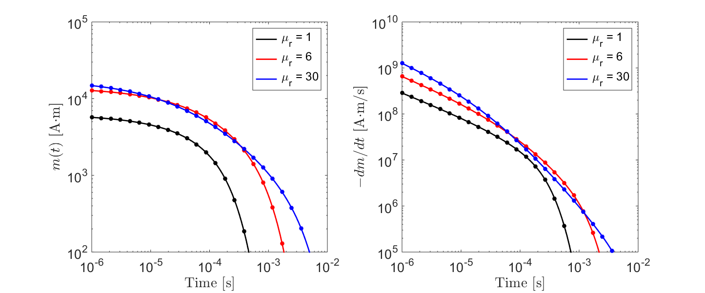
Fig. 144 Transient response from a conductive and permeable sphere for several relative permeabilities.

Impulse Response

The impulse response for a conductive and magnetically permeable sphere can be obtained by the following properties of the convolution:

(481)\[\chi (t) = \frac{d}{dt} \Big [ \chi (t) \otimes u(t) \Big ] = \frac{d}{dt} \mathcal{L}^{-1} \Bigg [ \frac{\chi(s)}{s} \Bigg ]\]

The above inverse Laplace transform was solved to obtain the step-on response in Eq (475), thus:

(482)\[\begin{split}\begin{align} \chi (t) &= \frac{d}{dt} \Bigg [ \frac{3}{2} \Bigg ( \frac{2 (\mu_r - 1)}{\mu_r + 2} - 6\mu_r \, \sum_{n=1}^\infty \frac{ e^{-\xi_n^2 t/\beta^2}}{(\mu_r + 2)(\mu_r - 1)+\xi_n^2} \Bigg ) u(t) \Bigg ]\\ &= Q \, \delta (t) + \, \frac{3}{2} \Bigg ( \frac{6 \mu_r}{\beta^2} \sum_{n=1}^\infty \frac{ \xi_n^2 \, e^{-\xi_n^2 t/\beta^2}}{(\mu_r + 2)(\mu_r - 1)+\xi_n^2} \Bigg ) u(t) \end{align}\end{split}\]

where

(483)\[Q = \frac{3}{2} \Bigg ( \frac{2 (\mu_r - 1)}{\mu_r + 2} - 6\mu_r \, \sum_{n=1}^\infty \frac{ 1 }{(\mu_r + 2)(\mu_r - 1)+\xi_n^2} \Bigg )\]

\(Q\) happens to be the convolution of \(\chi (t)\) and \(u(t)\), evalutated at \(t=0\). This can be checked using Eq. (475). By the initial value theorem of the Laplace transform:

(484)\[Q = \big [\chi (t) \otimes u(t) \big ] \Big |_{t=0} = \lim_{s \rightarrow \infty} \chi(s) = - \, \frac{3}{2}\]

Therefore, the impulse response for a conductive and permeable sphere is:

(485)\[\chi (t) = - \, \frac{3}{2} \delta (t) + \, \frac{3}{2} \Bigg ( \frac{6 \mu_r}{\beta^2} \sum_{n=1}^\infty \frac{ \xi_n^2 \, e^{-\xi_n^2 t/\beta^2}}{(\mu_r + 2)(\mu_r - 1)+\xi_n^2} \Bigg ) u(t)\]