Synthesis: Harmonic and Transient responses

Purpose

Provide integrated understanding of harmonic and transient EM responses using the simple circuit model.

(Source code, png, hires.png, pdf)

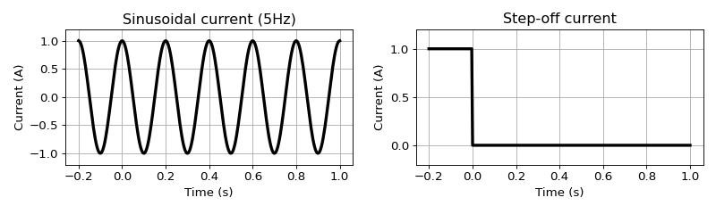
Harmonic and transient responses are respectively oscillating and decaying in time, and they are due to sinusoidal and step (either on or off) current. If we have full band of frequency or time, then we can obtain one from the other. However, in practice our measured band is limited hence each response can sense different information of the earth. Often, harmonic one is called frequency domain EM and transient one is called time domain EM.

An important feature in the harmonic case was the normalization of secondary EMF with the primary EMF, and this is same has the ratio between secondary and primary magnetic field. In contrast, for the transient response, this normalization was not available because the primary EMF is zero when \(t>0\), and this feature emphasized the importance of scale in transient response.

From the asymptotic behavior of the response function in frequency domain we defined Resistive and Inductive limit. Here, we revisit these with more integrated manner. In addition, we also briefly discuss different types of the measured response: magnetic field and EMF.

Inductive Limit

This limit indicates the stage of induction process where all secondary currents are concentrated at the surface of the isolated body to oppose the change in the normal component of the primary field. At this instant current has not penetrated into the conductor and the inductive limit is dependent only on the geometry of the target. We work through this limit in both frequency and time domain.

Response function in frequency domain can be written as

\[Q(\omega) = \frac{\imath \omega \tau}{1+\omega\tau}\]

Inductive limit is when \(\omega\) goes to \(\infty\):

\[\lim_{\omega \rightarrow 0 } Q = 1\]

Then the measured EM response will be

\[\frac{H^s}{H^p}=CQ = C,\]

where \(C\) is the coupling coefficient (only dependent on geometry of the loops). For transient response this will correspond to time at zero because the response function with step-on current, \(q_{on}(t)\) will be

\[\lim_{t \rightarrow 0 } q_{on}(t) = \lim_{t \rightarrow 0 } e^{-t/\tau} = 1, \ t>0\]

This will be directly connected to the secondary magnetic field with the step- on current, \(h^s_{on}(t)\):

\[h^s_{on}(t) = CH^p q_{on} (t)\]

and the early time limit will be

\[\lim_{t \rightarrow 0 } h^s_{on}(t) = CH^p\]

Therefore, with the step current excitation for the secondary magnetic field inductive limit can be reached at the early time limit.

Note

This is not true for the secondary EMF, \(\mathcal{E}^s\).

Resistive Limit

At this limit the induced currents have penetrated the body fully, and conductivity information can be extracted as well as geometry.

The restive limit is defined in the frequency domain as the slope of the response function as frequency approaches to zero:

\[\lim_{\omega \rightarrow 0} \frac{1}{\imath}\frac{\partial Q(\omega)}{\partial \omega} = \tau,\]

which has the exact time-domain equivalent

\[\int_{0}^{\infty}q_{on}(t) = \tau\]

Effectively, harmonic and transient response at the resistive limit can be written as

\[\text{Resistive limit:}\ \frac{H^s}{H^p} = \imath \omega \tau C\]

\[h^s_{on} = C H^p \tau\]

Magnetic field vs. EMF

When illustrating Inductive and Resistive limits, we use magnetic field as our response because the secondary magnetic field was compatible to define both limits in time domain. However, often we measure EMF at the Rx loop hence, we need to clarify their relationship.

Faraday’s law in integral form can be written as

\[\mathcal{E}(t) = \int_{S} -\mu_0 \frac{\partial \mathbf{h}}{\partial t} \cdot d \mathbf{S}\]

Since integration is spatial operation, time behavior of the EMF will be same as the time derivative of magnetic field with the negative sign.

A key feature of transient response is absence of the primary field when \(t>0\). This is only true for the magnetic field when step-off current is used. However, for the EMF it is true for both currents.

Note

EMF can loosely be considered as time derivative of the magnetic field with the negative sign.