Layered Earth

Purpose

In previous section, we used a half-space model, and due to zero conductivity of the air layer, conduction currents cannot flow, and this made drastic changes in EM fields. More complexity can be made when the earth medium is layered, have different conductivity values because of reflection and refraction of EM waves at layer interfaces. By using a layered earth model having four layers including the air layer, we explore how conductivity contrasts in these layered medium can distort EM fields, and data measured at an Rx location.

We use a similar setup used in the previous section, but fix the Tx height to \(z\) = 30 m. Fig. 112 shows a setup for the layered-earth model. The thickness of the first and second layer will be fixed to \(h_1\) = 6 m, and \(h_2\) = 12 m, respectively. All simulation results will be shown following can be reproducible from the Harmonic layered earth app accessible through this link:

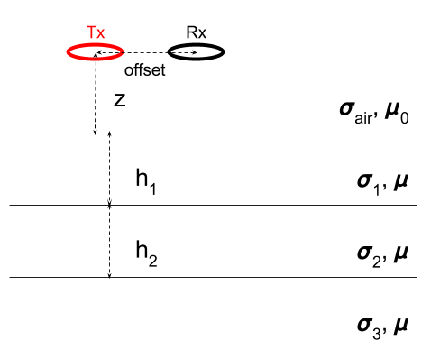
Fig. 112 A loop source in a layered-earth. \(\sigma_{air}\) is conductivity of the air layer, and suscript of conductivity stands for i-th layer. \(h_1\) and \(h_2\) correspondingly indicate thickness of 1st and 2nd layers. \(z\) and offset correspondingly indicate Tx height (m) and Tx-Rx offset (m).

Fields

With the above setup, here we present how EM fieids behave upon different conductivity structure of the layered-earth. We first perform a simulation for the half-space case when \(\sigma_1=\sigma_2=\sigma_3=\) 0.01 S/m with \(f\) = 1000 Hz. Fig. 113 a and b show imaginary part of secondary magntic flux (\(\mathbf{B}_s\)) and electric field in \(y\)-direction (\(E_y\)). Secondary magnetic flux flowing downward show anomalous amplitude along 1st and 2nd layers. Induced electric field are circular and at high amplitude regions are along 2nd and 3rd layers.

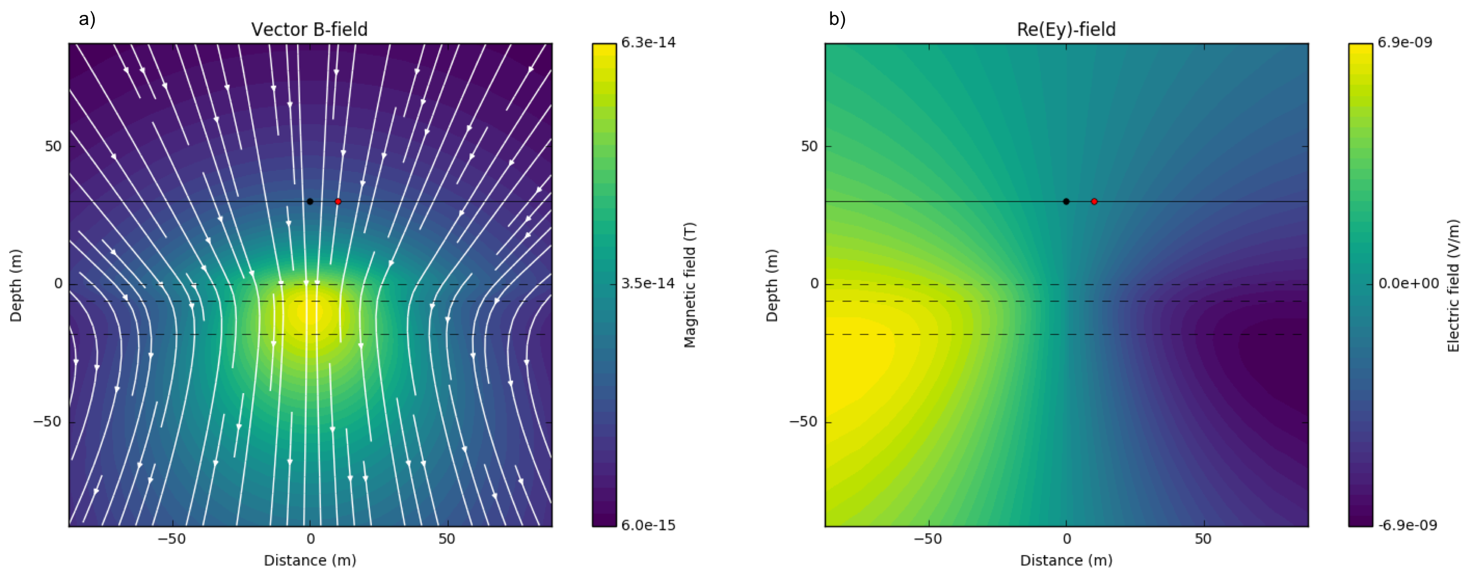
Fig. 113 Imaginary part of secondary magnetic flux a) and electric field in \(y\)-direction b). \(\sigma_1 = \sigma_2 = \sigma_3=\) 0.01 S/m; \(f\) = 1000 Hz.

Now we alter conductivity of the third layer, \(\sigma_3\) as 0.001 S/m, implying resistive basement. This effectively makes conductivity constrast between 2nd and 3rd layer. Fig. 114 a and b show imagniary part of \(\mathbf{B}_s\) and \(E_y\), respectively. At 3rd layer, amplitude of \(\mathbf{B}_s\) is decreased. Similarly high amplitude of electric field is localized to first and second layers. Less EM induction occurs when earth include resistive basement, but still this distorts EM fields suggesting potential to detect and delineate top boundary of the resistive basement.

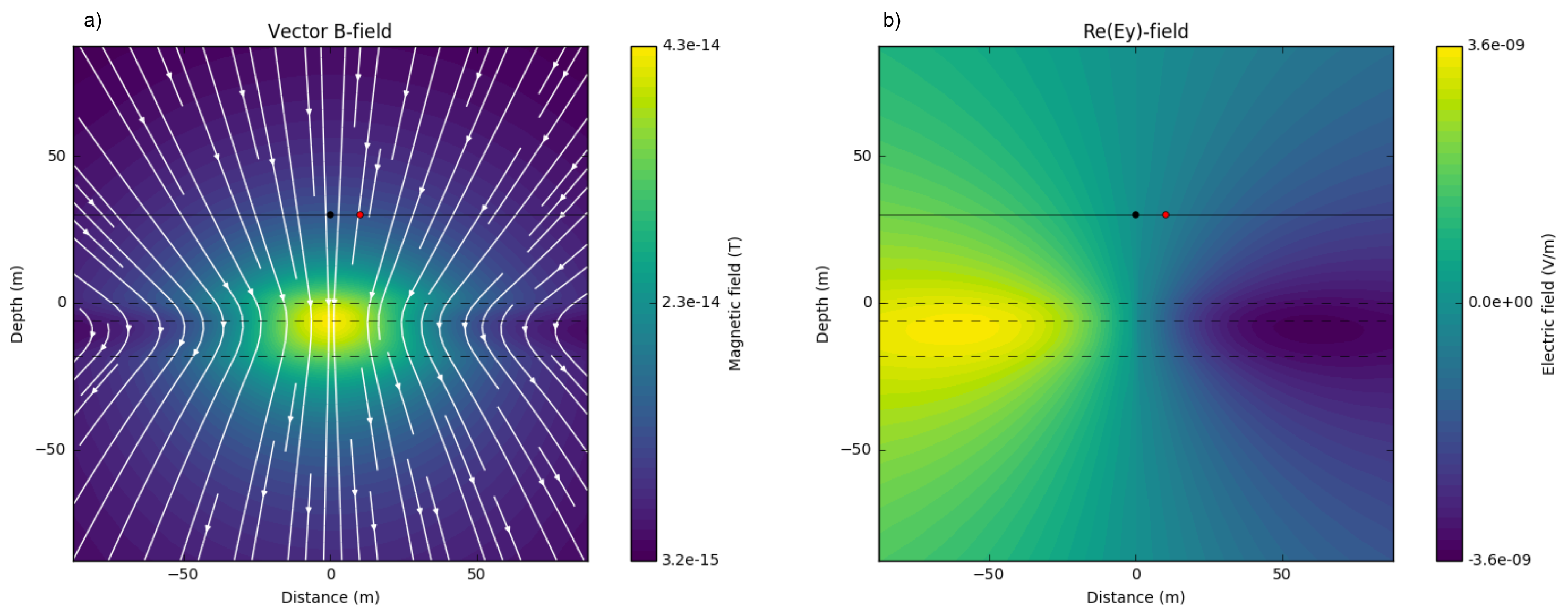
Fig. 114 Imaginary part of secondary magnetic flux a) and electric field in \(y\)-direction b). \(\sigma_1=\sigma_2 =\) 0.01 S/m and \(\sigma_3 =\) 0.001 S/m; \(f\) = 1000 Hz.

Often conductive cover could exists hence, we alther the first layer conductivity, \(\sigma_1\) as 0.1 S/m. This conductivey cover will generate significant eddy currents. Fig. 115 show a and b show imaginary part of \(\mathbf{B}_s\) and \(E_y\) for this case. High amplitude of \(\mathbf{B}_s\) is localized to the center of the first layer, and this causes significant bending of flux lines at each side. Induced electric field is also more localized to the first layer. Due to this strong EM induction effects at the first layer, resolving 2nd and 3rd layer conductivity will be challenging.

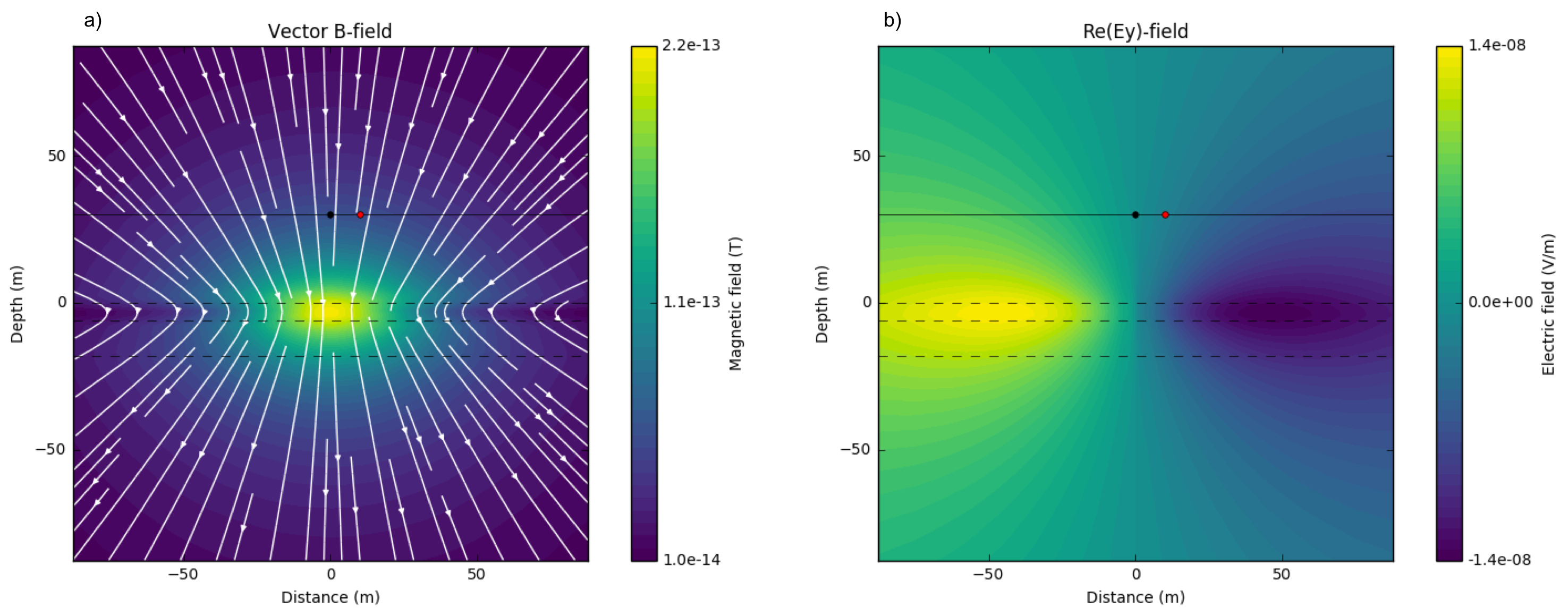
Fig. 115 Imaginary part of secondary magnetic flux a) and electric field in \(y\)-direction b). \(\sigma_1 =\) 0.1 S/m, \(\sigma_2 =\) 0.01 S/m and \(\sigma_3 =\) 0.001 S/m; \(f\) = 1000 Hz.

In contrast, resistive cover can exists, and for this case injecting currents using grounded source (e.g. DC) is hard. Hence using an inductive source can be effective to find conductive layer below this resistive cover. Fig. 116 a clearly shows high amplitude of magnetic flux at 2nd layer, which is conductive compared to the others. Similarly, amplitude of electric field at 2nd layer is higher than that at other two layers implying that we may resolve this conductive layer below the resistive cover.

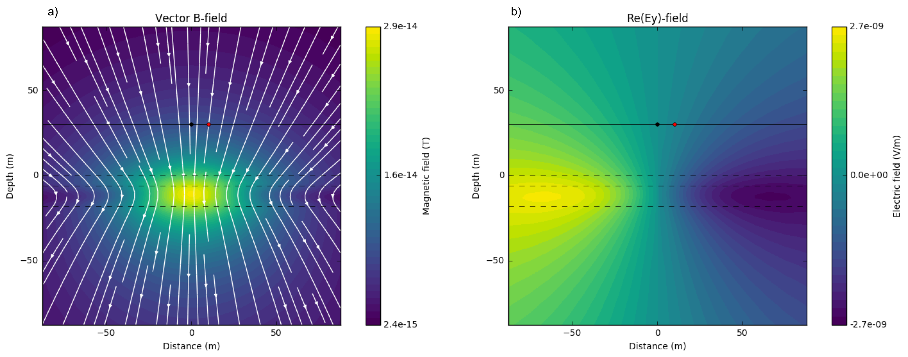
Fig. 116 Imaginary part of secondary magnetic flux a) and electric field in \(y\)-direction b). \(\sigma_1 =\) 0.1 S/m, \(\sigma_2 =\) 0.001 S/m and \(\sigma_3 =\) 0.001 S/m; \(f\) = 1000 Hz.

Data

Using the same four models: a) half-space, b) resistive basement, c) conductive cover, and d) resistive cover used to describe EM fields, here we present corresponding \(B_z\) data at the Rx location, which is 10 m apart from the Tx. Fig. 117 a-d correspondingly show the measured \(B_z\) data for above four models. Compared to the half-space model, when resistive basement exists, response of the basement model is smaller (< 10 KHz). Conductive cover makes the most drastic changes even in the data due to significant EM induction effects. For instance, peak of the imaginary part can clearly be observed for the conductive cover models, whereas recognizing peak of imaginary part is hard for other three models. Also, amplitude of responses are overall increased. Responses from the resistive cover model show the smallest amplitude. Also, difference from the basement model can clearly be recognized from 1000 Hz - 10 KHz.

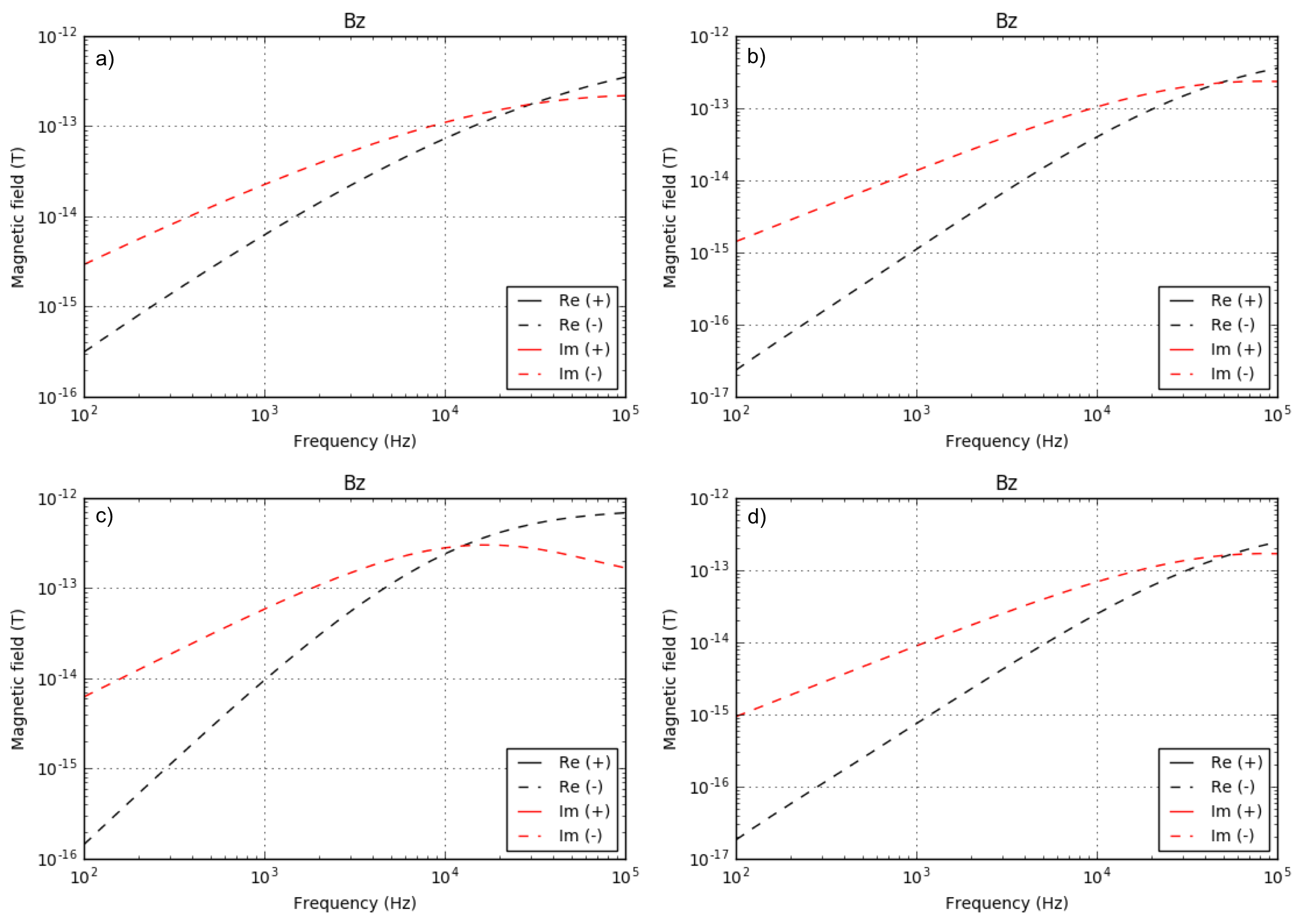
Fig. 117 Real and imaginary part of secondary \(B_z\) data at \(z`=30 m and :math:`x\) = 10 m. a) Half-space model (\(\sigma_1=\sigma_2=\sigma_3\) = 0.01 S/m), b) basement model (\(\sigma_1=\sigma_2\) = 0.01 S/m and \(\sigma_3\) = 0.001 S/m), c) conductive cover model (\(\sigma_1\) = 0.1 S/m, \(\sigma_2\) = 0.01, and \(\sigma_3\) = 0.001 S/m), and d) resistive cover model (\(\sigma_1\) = 0.001 S/m, \(\sigma_2\) = 0.01, and \(\sigma_3\) = 0.001 S/m). Red and black lines distinguish real and imaginary part of the data, and solid and dashed line distigusih positive and negative values.