Derivation of Interface Conditions

Here, we derive the interface conditions for fields \(\mathbf{e}\) and \(\mathbf{h}\) as well as for fluxes \(\mathbf{j}\), \(\mathbf{d}\) and \(\mathbf{b}\) according to Griffiths ([Gri99]). This can be accomplished by using Maxwell’s equations in integral form in the time-domain, where:

(75)\[\oint_S \mathbf{d} \cdot d \mathbf{a} = Q_f\]

(76)\[\oint_S \mathbf{b}\cdot d \mathbf{a} = 0\]

(77)\[\oint_C \mathbf{e} \cdot d\mathbf{l} = - \int_S \frac{\partial \mathbf{b}}{\partial t} \cdot d\mathbf{a}\]

(78)\[\oint_C \mathbf{h} \cdot d\mathbf{l} = \int_S \bigg ( \mathbf{j} + \frac{\partial \mathbf{d}}{\partial t} \bigg ) \cdot d\mathbf{a}\]

Recall that \(Q_f\) and \(\mathbf{j}\) are the total enclosed free charge and free current density, respectively. The fields and fluxes are related through the following constitutive relationships:

(79)\[\mathbf{j} = \sigma \mathbf{e},\]

(80)\[\mathbf{d} = \varepsilon \mathbf{e},\]

(81)\[\mathbf{b} = \mu \mathbf{h},\]

where \(\sigma\) denotes the electric conductivity, \(\varepsilon\) denotes the dielectric permittivity and \(\mu\) denotes the magnetic permeability.

Components Normal to the Interface

Here, we consider components of the fields and fluxes which are normal to the interface.

Electric Displacement

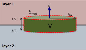
Fig. 39 Gaussian pillbox.

Although it may seem counter-intuitive, we will first derive the interface condition for normal components of the electric displacement. Consider an extremely small Gaussian pillbox of height \(h\) and cross-sectional area \(S_{\text{top}} = \pi r_{\text{top}}^2\) (Fig. 39). By applying Eq. (75) to our Gaussian pillbox, we obtain:

\[\int_0^{2\pi}\int_0^{r_{\text{top}}} d_1^\perp ~drd\theta - \int_0^{2\pi}\int_0^{r_{\text{top}}} d_2^\perp ~ dr d \theta + \int\limits_{-h/2}^{h/2}\int\limits_0^{2\pi} d^\parallel ~ d \theta dz = Q_f\]

where \(d_{1}^\perp\) and \(d_{2}^\perp\) are the components of the electric displacement normal to the top and bottom of the pillbox, respectively. The radial component (parallel to the interface) is denoted by \(d^\parallel\). Since the pillbox is extremely small, we can assume that \(d_{1}^\perp\) and \(d_{2}^\perp\) are constant over the top and bottom of the pillbox, respectively. Under this assumption, the previous expression can be simplified to:

(82)\[d_{1}^\perp S_{\text{top}} - d_{2}^\perp S_{\text{top}} + \int\limits_{-h/2}^{h/2}\int\limits_0^{2\pi} d^\parallel ~ d \theta dz = Q_f.\]

If we take the limit as \(h\rightarrow 0\) while letting \(S_{\text{top}}\) remain fixed, the integral term on the left hand side of Eq. (82) vanishes. Additionally, as the vertical dimension of the pillbox goes to zero, the total enclosed free charge \(Q_f\) becomes the product of a free surface charge density \(\tau_f\) and the area of the top of the pillbox; assuming the distribution of surface charges is constant. This results in the following expression:

\[d_{1}^\perp S_{\text{top}} - d_{2}^\perp S_{\text{top}} = \tau_f S_{\text{top}}\]

Dividing both sides by the top area of the pillbox, the interface condition for normal components of the electric displacement are given by:

(83)\[d_{1}^\perp - d_{2}^\perp = \tau_f\]

Thus, the normal component the electric displacement is discontinuous at the interface. Furthermore, the discontinuity is associated with an accumulation of electrical charges.

Electric Field

To obtain the interface condition for normal components of the electric field, we can combine Eqs. (80) and (83). Thus:

(84)\[\varepsilon_1 e_{1}^\perp -\varepsilon_2 e_{2}^\perp = \tau_f\]

Current Density

To obtain the interface condition for normal components of the electric current density, we can combine Eqs. (79) and (84). Thus:

(85)\[\frac{\varepsilon_1}{\sigma_1} j_{1}^\perp - \frac{\varepsilon_2}{\sigma_2} j_{2}^\perp = \tau_f\]

In the case where there is no difference in dielectric properties across the interface, this equation simplifies to the following:

(86)\[\frac{j_{1}^\perp}{\sigma_1} - \frac{j_{2}^\perp}{\sigma_2} = \frac{\tau_f}{\varepsilon_0}\]

Special Cases: Steady-State Current

To examine this case, let us consider the continuity equation for conservation of charge:

(87)\[\int_A \mathbf{j} \cdot d\mathbf{a} = -\frac{dQ_f}{dt}\]

In the steady-state, the density of free charge on the interface is static in time. Thus the right hand side of the previous equation is zero. If we use the Gaussian pillbox from Fig. 39 and follow the same arguments used to derive interface conditions for \(d^\perp\), we find that:

(88)\[j_1^\perp = j_2^\perp\]

Thus in the steady state, the normal component of the current density is continuous across the interface. If we let \(j_1^\perp = j_2^\perp = j^\perp\), the interface condition for the electric current density in the absence of dielectrics simplifies to:

(89)\[\bigg ( \frac{1}{\sigma_1} - \frac{1}{\sigma_2} \bigg ) j^\perp = \big ( \rho_1 - \rho_2 \big ) j^\perp = \frac{\tau_f}{\varepsilon_0}\]

where \(\rho = 1/\sigma\) is the electric resistivity. Although accumulation of electrical charge is complete in this case, it is important to note that the difference in electrical properties across the interface is responsible for the accumulation of electrical charge.

Magnetic Flux Density

The interface condition for the normal component of the magnetic flux density is derived from Eq. (76); i.e. Gauss’s law for magnetic fields. For this, we may follow the exact same argument used to obtain interface conditions for the electric displacement. However, since the right hand side of Eq. (76) is always zero, the interface condition for the normal component of the magnetic flux density is given by:

(90)\[b_{1}^\perp - b_{2}^\perp = 0\]

Therefore, normal components of the magnetic flux density are continuous across interfaces.

Magnetic Field

To obtain the interface condition for normal components of the magnetic field, we can combine Eqs. (81) and (90). Thus:

\[\mu_1 h_{1}^\perp -\mu_2 h_{2}^\perp = 0\]

Components Tangential to the Interface

Here, we consider components of the fields and fluxes which are tangential to the interface.

Electric Field

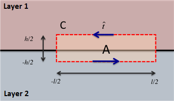
Fig. 40 Gaussian rectangle.

Although it may seem strange given the previous ordering, we will first derive the interface condition for tangential components of the electric field. Consider a Gaussian rectangle of height \(h\), width \(l\) and area \(A\) (Fig. 40). The surface of this rectangle is perpendicular to the interface.

We begin by applying Eq. (77) to our rectangle. Assuming the rectangle is small enough such that the tangential electric field is constant along both horizontal edges, we obtain the following:

(91)\[\oint_C \!\mathbf{e}\cdot d\mathbf{l} = e_{1}^\parallel \, l - e_{2}^\parallel \, l + \int_{-h/2}^{h/2} e^\perp (x \! =\! -l/2) ~dz - \int_{-h/2}^{h/2} e^\perp (x \! = \! l/2) ~dz = - \!\int_A \frac{\partial \mathbf{b}}{\partial t}\cdot d \mathbf{a}\]

where \(e_{1}^\parallel\) and \(e_{2}^\parallel\) are the tangential components of the electric field on the top and bottom edges of the Gaussian rectangle, respectively. Normal components of the electric field are denoted by \(e^\perp\).

If we take the limit \(h \rightarrow 0\) while leaving the width \(l\) fixed, the integrals on the left hand side of Eq. (91) go to zero. Additionally, this limit causes the surface area of the rectangle to go to zero, thus the integral on the right hand side of Eq. (91) is also zero. Thus:

(92)\[e_{1}^\parallel \, l - e_{2}^\parallel \, l = 0\]

Dividing the previous equation by \(l\), we obtain the interface condition for tangential components of the electric field:

(93)\[e_{1}^\parallel - e_{2}^\parallel = 0.\]

The tangential component of the electric field is continuous across the interface. As a result, tangential components of the electric field are not responsible for any build-up of electrical charges at the interface.

Electric Displacement

To obtain the interface condition for tangential components of the electric displacement, we can combine Eqs. (80) and (93). Thus:

(94)\[\frac{ d_{1}^\parallel}{\varepsilon_1} - \frac{d_{2}^\parallel}{\varepsilon_2} = 0\]

Current Density

To obtain the interface condition for tangential components of the electric current density, we can combine Eqs. (79) and (93). Thus:

(95)\[\frac{ j_{1}^\parallel}{\sigma_1} - \frac{j_{2}^\parallel}{\sigma_2} = \rho_1 j_1^\parallel - \rho_2 j_2^\parallel = 0\]

where \(\rho = \sigma^{-1}\) is the electric resistivity.

Magnetic Field

The interface condition for the tangential component of the magnetic field is derived from Eq. (78); i.e. the Ampere-Maxwell equation. Here, we can follow the exact same arguments used to obtain interface conditions for the electric field. In this case however, we must also address the integral term which contains the free current density such that:

(96)\[I_f = \int_S \mathbf{j} \cdot d \mathbf{a}\]

where \(I_f\) is the total enclosed free current. By taking the limit \(h \rightarrow 0\), the Ampere-Maxwell equation applied to the Gaussian loop becomes:

(97)\[\oint_C \mathbf{h}\cdot \mathbf{d}\mathbf{l} = h_{1}^\parallel \, l - h_{t}^\parallel \, l = I_f\]

Like the right hand side of Eq. (91), the flux term containing the electric displacement goes to zero as the area of the loop goes to zero. This however, is not the case for the enclosed free current. As \(h \rightarrow 0\), there is still free current which flows along the interface. The free surface current is the product of a surface current density \(K_f\) and the width of the loop; assuming \(K_f\) is constant along the interface. Thus:

(98)\[h_{1}^\parallel \, l - h_{2}^\parallel \, l = K_f l\]

Dividing the previous expression by the width of the loop, the interface condition for the tangential component of the magnetic field is given by:

(99)\[h_{1}^\parallel - h_{t}^\parallel = K_f\]

Therefore, the tangential component of the magnetic field is discontinuous at the interface. Furthermore, the discontinuity of the magnetic field is related to a free surface current density which flows along the interface.

Magnetic Flux Density

To obtain the interface condition for tangential components of the magnetic flux density, we can combine Eqs. (81) and (99). Thus:

(100)\[\frac{b_{1}^\parallel}{\mu_1} - \frac{h_{t}^\parallel}{\mu_2} = K_f\]