Interpretation

Purpose

To show how DCR data are processed and inverted to reveal meaningful information about the earth structure. This is demonstrated on data generated from a buried prism and the two-sphere problem.

Apparent Resistivities

Plotting apparent resistivities, as pseudosections or in plan-view maps, is informative. The images are useful for recognizing data outliers, bad electrodes, and validating normalizations that might have been applied to the data. In addition, they sometimes provide valuable information about earth structure.

As an illustration, Fig. 160 (a) shows an earth model consisting of a single prism (\(\rho=10\; \Omega \cdot m\)) buried in a uniform halfspace (\(\rho= 100\; \Omega \cdot m\)). A dipole-dipole survey is carried out along a line that passes directly above the conductive prism. The resulting pseudosection is shown in Fig. 160 (b). The prism is manifested as a region of lower apparent resistivity in the center of the image and there are wings extending outwards and downward. The apex of the image can be used to estimate the horizontal location of the prism but the depth to the body is less evident since the vertical scale of the pseudosection is in n-values and not in meters.

Despite the above success, the situation worsens if the earth is more complex. This is illustrated in Fig. 160 (c) where some near-surface inhomogeneities are added. The same dipole-dipole survey is carried out and resultant pseudosection is shown in Fig. 160 (d). The response of the prism is masked and attempting to infer existence and location of the prism is extremely challenging.

This example can be downloaded here.

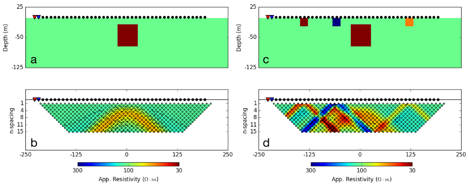
Fig. 160 : (a) Vertical section through a simple conductive prism (\(\rho=10 \;\Omega \cdot m\)) buried in a homogeneous halfspace \(\rho=100 \;\Omega \cdot m\). Source and receiver locations for a dipole-dipole survey are shown for reference. (b) Pseudosection of apparent resistivity calculated from the synthetic DCR survey. (c) Vertical section through a more complicated resistivity model with near-surface inhomogeneities added and (d) resulting pseudosection of apparent resistivity.

Gradient array surveys are often used in reconnaissance modes and it is insightful to repeat the above analysis with a representative example. A plan view of the resistivity model and electrode geometry is shown in Fig. 161 (a). The survey consists of a grid of 13 x 13 receivers located between a 450 meter dipole current source. Each receiver is a 20 meter dipole. The corresponding apparent resistivity map is shown in Fig. 161 (b). An estimate of the horizontal location of the center of the prism can be obtained, but again there is no quantitative information about the depth.

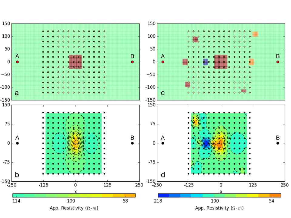
Fig. 161 : (a) Bird-eye view of gradient array survey over a simple conductive prism model (\(\rho= 10\; \Omega \cdot m\)) buried in a uniform halfspace (\(\rho= 100\; \Omega \cdot m\)) and (b) corresponding apparent conductivity map. By simple inspection of the data map, it is easy to locate the center of the conductive anomaly. (c) The experiment is replicated with a more complicated conductivity model with near-surface inhomogeneities added. Direct interpretation of the resulting apparent resistivity map (d) is challenging.

Contaminating the model by adding some conductive and resistive features (Fig. 161 (c)) leads to an apparent resistivity map that is very complicated and in which the signal of the prism is masked (Fig. 161 (d)). To obtain information about the electrical conductivity we need to invert the data.

Inversion of DCR data

The DCR data are inverted using a standard Gauss-Newton framework. This is outlined in Inversion. The data are the measured voltages and the goal is to find an electrical conductivity that satisfactorily reproduces these data and agrees with a priori geologic structure and petrophysical constraints.

To illustrate the importance of inverting the data, we return to the thematic 2-sphere problem. Although the geology is 3D, we first invert the data using a 2D inversion algorithm. Parameters used for the inversion of the dipole-dipole data (Fig. 162 (b)) are provided in Table 3.

Table 3 : 2D Inversion parameters

Number of sources	43
Number of data	540
Data uncertainties	\(2\%|d| (percentage) + 2 \times 10^{-5} V\) (floor)
Mesh Size	\(10 \times 10 \times 10\) meters
Reference conductivity	\(0.01\) S/m
Regularization Scales ( \(\alpha_s, \alpha_x,\alpha_y,\alpha_z\) )	\(0.01, 1, 1, 1\)

Fig. 162 (c) presents the recovered 2D conductivity model after convergence of the algorithm.

Important comments:

1. Even though there are no contaminating near-surface blocks the pseudosection does not clearly indicate two bodies. This is in contrast to Fig. 160 (a) where a single prism was clearly identified in the pseudosection.

2. The two spheres are recovered but they have lower conductivity contrasts with respect to the halfspace than do the true spheres. This occurs for three reasons: (i) the inversion generates smooth models and this extends structures and reduces amplitudes; (ii) the true spheres extend into regions where there is limited depth of investigation; and (iii) the 2D inversion assumes that the structures are cylindrical.

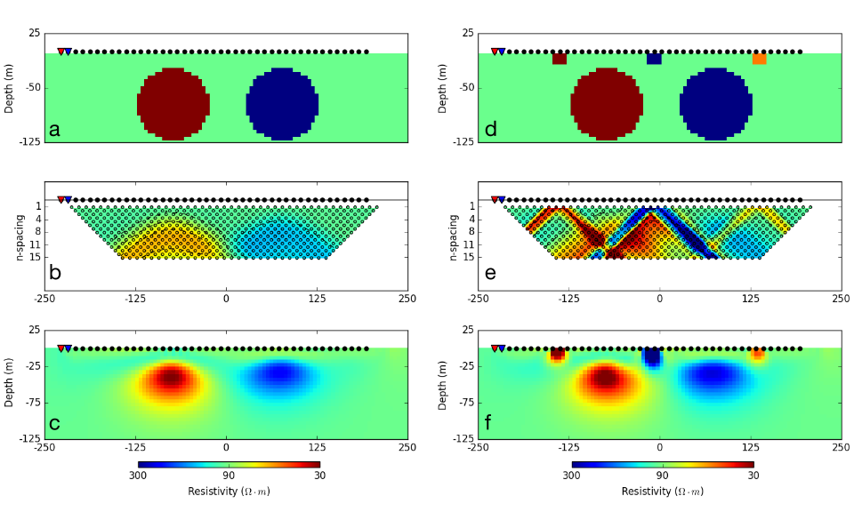
Fig. 162 : (a) Vertical section through a two-sphere model (\(\rho_1= 10\; \Omega \cdot m\) ; \(\rho_2= 1000\; \Omega \cdot m\)) buried in a homogeneous halfspace (\(\rho_0= 100\; \Omega \cdot m\)). (b) Corresponding pseudosection of apparent conductivity acquired from a dipole-dipole survey layout, 20 meter dipole spacing. (c) Recovered conductivity model from a 2D inversion. (d) Two sphere model with near-surface inhomogeneities. (e) pseudosection (f) Recovered model from 2D inversion.

Similar to the prism model example (Fig. 160), we repeat the experiment with the same survey setup but use a more complicated resistivity model that has near-surface inhomogeneities (Fig. 162 (d)). The resulting pseudosection (Fig. 162 (e)) is challenging to interpret visually. The 2D resistivity model recovered from the inversion ( Fig. 162 (f)) unravels the data complexity.

Important comments:

1. The pseudosection of data is complicated and dominated by the near-surface conductors.

2. The inversion recovers the contaminating surface conductors. It also recovers the two spheres with about the same fidelity as in the simple case.

This example can be downloaded here.

Depth of Investigation

The inverse problem is nonunique and the DCR data are sensitive to conductivity only in a region in the vicinity of the electrode array. Conductivity structures that exist outside this region are unreliable and likely artifacts of the inversion. There are several methods proposed in the literature to quantify this limits of this region for a specific DCR survey. The following example uses the Depth of Investigation (DOI) method proposed by [LO99].

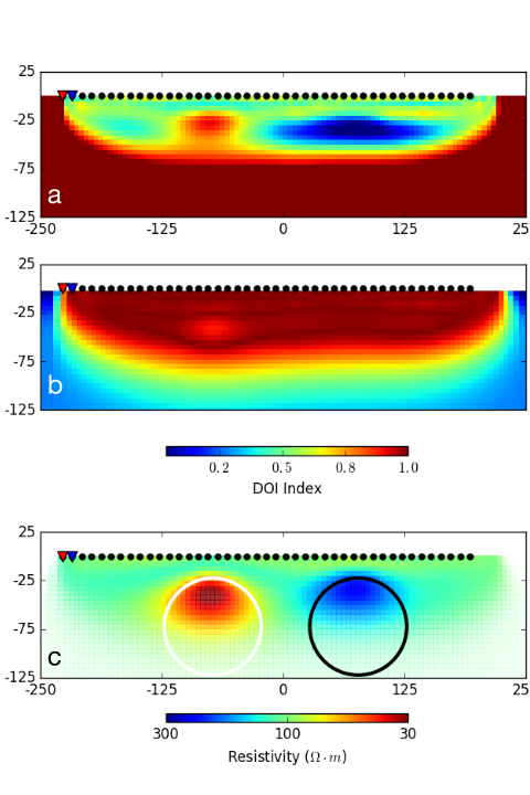
Fig. 163 : (a) Resistivity model obtained using a different reference halfspace (\(\rho= 10\; \Omega \cdot m\)) and (b) the calculated DOI index. (c) Preferred resistivity model presented in Fig. 162 (c) after applying the DOI mask.

In its simplest form, the DOI analysis requires the data to be inverted twice with all parameters the same except for the background conductivity. For the two-sphere example shown in Fig. 162 (c), the synthetic data is inverted a second time with a reference halfspace conductivity of \(10\; \Omega \cdot m\). Fig. 163 (a) shows the recovered 2D resistivity model. Note that the region away from the electrode locations returns to a value close to the reference model.

We now have a discretized volume of the Earth and two conductivity models that can equally reproduced the observed data. Let \(\sigma_1, \sigma_2\) be the conductivity values recovered at some location (x,z), a DOI index is calculated as:

\[DOI(x,y) = 1 - \big| \frac{\sigma_1(x,y) - \sigma_2(x,y)}{\sigma_1^{ref} - \sigma_2^{ref}} \big|\;,\]

where the DOI index will approach 1 for similar model values obtained with both inversions regardless of the chosen reference models \(\sigma_1^{ref}, \sigma_2^{ref}\). Conversely, the DOI will approach 0 where the recovered models return to their respective reference conductivities. Fig. 163 (b) presents the calculated DOI index for the two- sphere problem, showing a lower confidence over the bottom half of the domain. The DOI mask is applied to our preferred 2D model, presented in Fig. 163 (c), with transparency applied proportionally to the DOI index.

Downloads

Data, model and inversion files used in this page can be downloaded below:

Prism

Two_Spheres

Utilities: UBC-DC2D data viewer and model viewer